This is the forth and final post of a short series of posts on extreme events in financial time series. In the first post, we have introduced power-law theory to describe and extrapolate the chance of extreme price movements of the S&P500 index. In the second post, we took a closer look at how statistical moments may become infinite in the presence of power-law tails, rendering common estimators useless. In the third post, we have seen how infinite kurtosis makes GARCH risk models fail on out-of-sample data. In this post, we turn to Markowitz’s Modern Portfolio Theory and show how the heavy tails of financial return distributions drastically increase the uncertainty in portfolio allocation weights.
You can access an interactive Python version of this blog post here. It is powered by JupyterLite and runs directly in your browser without any install or config!
In 1954, Harry Markowitz received his PhD in economics for a work on portfolio theory. His work was the founding stone of Modern Portfolio Theory and back then it was such a novelty that during his PhD defense, Milton Friedman argued that the work does not really belong to the field of economics (as Markowitz explained in his Nobel lecture in 1990). Markowitz argued that for a given level of volatility, there is a set of allocation weights for the assets within a portfolio that yield a maximum portfolio excess return (compared to a risk-free asset). If you scan through a range of volatility values and compute the maximum portfolio return by obtaining the optimal allocation weights, you will get the set of efficient portfolios, also called the efficient frontier. One point on this frontier is of special interest in many cases, it is the point of maximum Sharpe ratio.
The Sharpe ratio is an often criticized but also often used metric to evaluate the performance of a portfolio or financial assets in general, such as hedge funds or ETFs. It is defined as:
$$
S = \frac{\mu – \mu_{\text{rf}}}{\sigma}
$$
Here, $\mu$ denotes the annualized portfolio return, $\mu_{\text{rf}}$ denotes the annualized risk-free return, and $\sigma$ denotes the annualized portfolio volatility. Assuming a zero risk-free rate ($\mu_{\text{rf}} = 0$), the Sharpe ratio can be interpreted as a signal-to-noise ratio known in Physics and Engineering: by maximizing the Sharpe ratio, we find the best trade-off between maximizing our returns (the signal) and minimizing volatility (the noise).
If our portfolio consists of $n$ financial assets with the expected returns $\vec{\mu} = (\mu_1, …, \mu_n)$, with the covariance matrix $\Sigma$ that holds the information about volatility and correlations between assets, and with the allocation weight vector $\vec{w} = (w_1, …, w_n)$ (normalized to unity: $\sum_{i=1}^n w_i = 1$), then the Sharpe ratio can be computed as follows in the context of Modern Portfolio Theory. Note that we always assume $\mu_{\text{rf}} = 0$ from hereon:
$$
S(\vec{w}) = \frac{\vec{w}.\vec{\mu}}{\sqrt{\vec{w}.\Sigma.\vec{w}^T}}
$$
To maximize the return relative to the volatility and obtain the maximum-Sharpe portfolio, we change the allocation weights until we find the set of weights $\vec{w}^*$ with the maximum Sharpe ratio:
$$
\vec{w}^* = \text{argmax}_{\vec{w}} ~ S(\vec{w})
$$
The underlying assumption behind Modern Portfolio Theory is that the joint distribution of log-returns of all assets in the portfolio can be fully characterized by a multi-variate Gaussian distribution. After the previous parts of this blog post series, we know this fallacy very well, and Modern Portfolio Theory has rightfully received harsh criticism for this lack of accounting for heavy tails, e.g. by Nassim Taleb:
After the stock market crash (in 1987), they rewarded two theoreticians, Harry Markowitz and William Sharpe, who built beautifully Platonic models on a Gaussian base, contributing to what is called Modern Portfolio Theory. Simply, if you remove their Gaussian assumptions and treat prices as scalable, you are left with hot air. The Nobel Committee could have tested the Sharpe and Markowitz models—they work like quack remedies sold on the Internet — but nobody in Stockholm seems to have thought about it.
— Nassim Taleb in The Black Swan: The Impact of the Highly Improbable (p.277)
In this post, want to illustrate the consequences of the Gaussianity assumption by simulating returns of two hypothetical stocks and trying to find the maximum-Sharpe allocation weights. As we shall see, heavy tails in the simulated return distributions introduce substantial uncertainty in the estimated allocation weights. This increased uncertainty is caused by the infinite kurtosis of real-world return distributions: if higher moments such as kurtosis become very large or infinite, the estimation of lower moments such as variance is destabilized. Variance and volatility as its square-root, however, are key ingredients in many finance models, and the estimation of model parameters thus may be severely affected by heavy tailed return distributions.
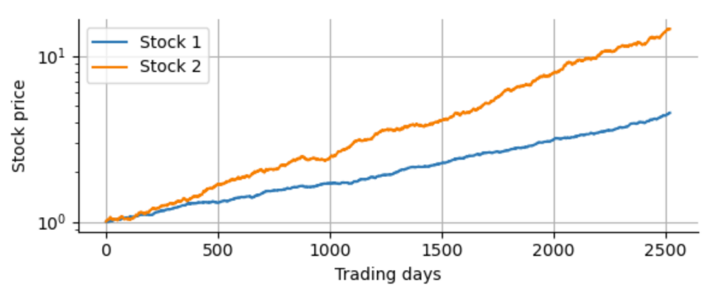
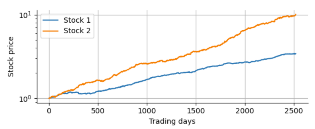
To simulate this destabilization of volatility, we first draw random numbers from a Gaussian distribution, enough to simulate 10 years worth of daily log-returns for two hypothetical stocks. We assign different positive expected returns and volatility to them. For simplicity, we assume zero correlation between the two assets:
Of course, in reality we do not know the true expected returns, or volatility values or correlations between the assets. So we have to estimate the expected return by the sample mean and the covariance matrix by the sample covariance. Note that there are more elaborate ways to estimate these parameters from historical data, such as shrinkage estimators for the covariance matrix or the Black-Litterman allocation model. These methods certainly improve upon sample estimates, but the general short-coming of Modern Portfolio Theory in the presence of heavy tails remains. To study and test different portfolio optimization techniques, we recommend to take a look at PyPortfolioOpt, a well-documented Python package that implements basic as well as elaborate methods for portfolio optimization and allows to test these methods with real data easily. For now, we stick to the sample estimates (and use a factor of 252 – the average number of trading days per year – to obtain the annualized expected return and covariance from the daily estimates).
Rather than using a real optimizer to find the allocation weights that maximize the Sharpe ratio, we simply scan through all possible weight combinations at an interval of 1%, starting at a portfolio that allocates 100% to stock 1 and 0% to stock 2, then 99% to stock 1 and 1% to stock 2, and so on. For each combination, we compute the portfolio returns and calculate the Sharpe ratio using the formula above. Finally, we select the allocation weights that attained the maximum Sharpe ratio. This is of course only a reasonable approach for two assets and quickly becomes intractable with more than two assets.
To get an idea of how accurately we can estimate the allocation weights based on 10 years of hypothetical daily returns, we now repeat this experiment, we re-draw new random returns, re-estimate expected returns and covariance matrix, and scan for the optimal weights. We do this 10000 times. Note that we only log the first allocation weight $w^*_1$ for each run without losing information since the second weight directly follows from normalization $w^*_2 = 1 – w^*_1$ (at least in our case of trading without leverage). Finally, we can plot a histogram of all the 10000 values we get for $w^*_1$:
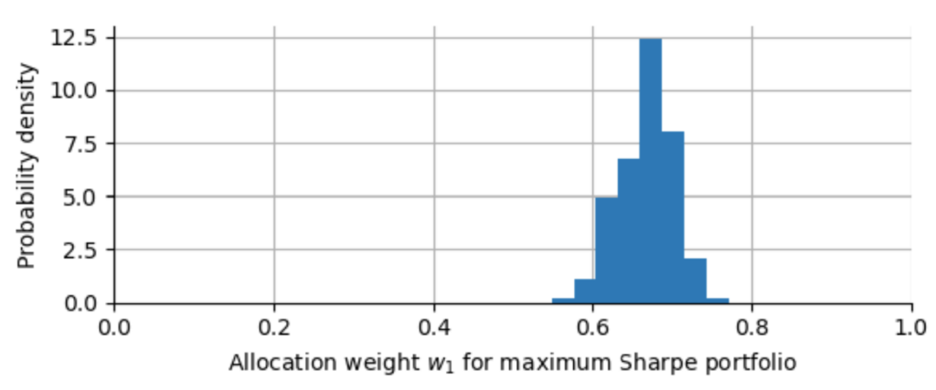
As we can see, the allocation for stock 1 varies roughly between 60% and 70%, based on 10 years of historical data. We can further quantify this by calculating the 5th and 95th percentile of all $w^*_1$-values. With 90% confidence, we will get an allocation between 61% and 72%.
Now let us repeat this experiment, but this time we replace the Gaussian distribution by a Student-t distribution with a power-law exponent of $\alpha=3.7$ (corresponding to a number of degrees of freedom of $\nu=2.7$), as we have estimated from daily S&P500 returns in the earlier blog post “The 23-sigma fallacy”. We leave the expected return and the volatility (measured by the standard deviation of the distribution) exactly the same. Note that the standard deviation of the standard t-distribution is defined as $\sqrt{\frac{\nu}{\nu-2}}$ in our case, so we have to correct for this scale factor when drawing random numbers from a standard t-distribution. Below, you can see a direct comparison of the Gaussian distributions used in the simulation above, and the t-distributions with matched mean and standard deviation.
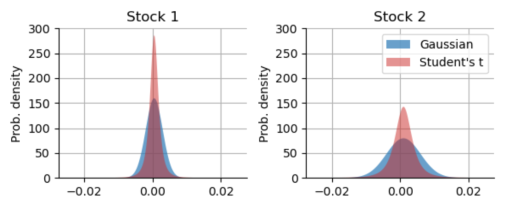
As we can easily see, the matched Student’s t-distributions actually produce more smaller return values. However, they also produce much more extreme values, but we cannot easily see that as the probability density values in the tails are very small! If we switch to a logarithmic scaling of the y-axis, the picture becomes more clear:
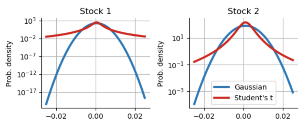
Now we can clearly see that, for example, the chance of a daily log-return of $-0.02$ for Stock 1 is $10^{10}$ times more likely assuming the t-distribution compared to the matched Gaussian distribution! Always take a look at distributions with a logarithmic scale of the probability density to get a clear picture of the tails. Using our matched t-distributions, we proceed as before and simulate hypothetical 10-year historical track records for our two uncorrelated stocks. Below you can see an example. Only by a close look you may spot that these cumulative return curves are actually a bit more ragged compared to the ones plotted above with the Gaussian returns. But the difference is subtle when looking at such a “zoomed-out” picture of a ten-year period:
Finally, to visualize the effect of the t-distribution on the estimation of allocation weights, we repeat our Monte Carlo experiment of simulating 10000 different 10-year histories and estimate the allocation weights in each of those 10000 cases. We then plot the distribution of $w^*_1$ and compare this distribution to the one obtained from the Gaussian simulations.
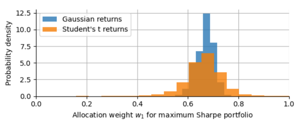
As we can see, the optimal allocation weight $w^*_1$ now fluctuates between 54% and 77%, roughly 2 times the width of the credible interval for the portfolio optimization that adhered to the assumption of Gaussianity! Even with a matched standard deviation of the Gaussian and the t-distribution, the infinite kurtosis of the t-distribution destabilizes the sample variance of our simulated return series and thus reduces the accuracy of our estimated allocation weights. While this example certainly does not uncover all weaknesses of Modern Portfolio Theory, it helps us to see how rather abstract effects like the instability of variance due to excess kurtosis ends up messing with widely employed financial models.
TAKE-HOME MESSAGE

The heavy tails of return distributions can greatly affect the outcome of established mathematical models in finance by drastically increasing parameter uncertainty! Using simulated returns based on Gaussian vs. heavy-tailed distributions can help to uncover limitations of financial models or help to find the minimum amount of data that is necessary to attain certain confidence, before a new model is actually put into production or even sees real data.
This post concludes a short series on extreme values in financial time series. If you have some basic Python coding experience, check out the interactive Python version of the blog post series that runs in your browser without any config/install. It is part of a course on risk mitigation that will be offered shortly by Artifact Research.
This blog post series was inspired by Nassim Taleb’s Statistical Consequences of Fat Tails: Real World Preasymptotics, Epistemology, and Applications (freely available via link). It is the first book of a mathematical parallel version of the Incerto series by Nassim Taleb on uncertainty.
Get notified about new blog posts and free content by following me on Twitter @christophmark_ or by subscribing to our newsletter at Artifact Research!
Hi Christoph,
Thanks for this series of post, especially the Student-t fitting.
On my side, I would have one comment re. “The underlying assumption behind Modern Portfolio Theory is that the joint distribution of log-returns of all assets in the portfolio can be fully characterized by a multi-variate Gaussian distribution.”
I find this is a frequent remark, but wrong, at least in the case of mean-variance analysis.
Ref. for instance “Risk-Return Analysis, Volume 1 / Markowitz with Blay”, chapters 1 and 2 and full discussion therein, but I can quote:
“The fact that Markowitz bases its support for mean-variance analysis on mean-variance approximations to expected utility is rarely cited.”
Cheers,
Roman
PS: That being said, and a a side note, from similar experiments and misc. readings, I remember that the gaussian approximation gets better and better at monthly/yearly levels for typical bonds/stocks. Do you confirm with this S&P500 dataset ?
Hi Roman,
thanks for pointing out the discussion on the assumptions underlying Modern Portfolio Theory, indeed I assumed that Gaussianity was required. This is a very interesting topic, I’ll probably make a follow-up on this some time soon and discuss this further!
And yes, the Gaussian approximation gets much better as we move to monthly or annual returns. In my opinion, this has two consequences: First, because there are fewer data points, you get a larger estimation error for expected return and volatility that has be accounted for. So the problem shifts a bit from estimation uncertainty because of the heavy tails to estimation uncertainty because of only few data points. I will prepare a post on a fully probabilistic version of metrics like the Sharpe ratio shortly.
Second, I think the better Gaussian approximation for more coarse-grained returns indeed is a point in favor of Modern Portfolio Theory as long as you are an investor that can definitely hold the assets for at least one whole period. If you are trading leveraged positions on margin then you are exposed to the daily price movements and then you need to carefully account for the heavy tails.
Again, thanks for your comments!
Cheers,
Chris
Are you writing the articles in your website yourself or you outsource them?
I am a blogger and having difficulty with content. Other bloggers told me I should
use an AI content writer, they are actually pretty good.
Here is a sample article some bloggers shared with me.
Please let me know what your opinion on it and should I go ahead and use AI – https://sites.google.com/view/best-ai-content-writing-tools/home