Probabilistic programming in finance: a robust Sharpe ratio estimate
In this post, we will develop a time-varying, probabilistic extension of the Sharpe ratio as a widely used performance metric for financial assets. In particular, we devise a Bayesian regime-switching model to capture different market conditions and infer the full distribution the Sharpe ratio as it changes over time using the probabilistic programming framework bayesloop. We show that by focusing on the left tail of the Sharpe distribution we can derive a robust point estimate of the Sharpe ratio that accounts for the additional uncertainty of short track records and avoids overestimating the Sharpe ratio in the case of temporary market rallies. Additionally, we show that the shape of the Sharpe distribution encodes the susceptibility of an asset to different market conditions and can thus help to identify resilient assets for long-term investments.
Adding new financial assets to existing portfolios or constructing portfolios from scratch requires performance metrics for individual assets to enable an objective choice. Commonly used metrics such as the Sharpe ratio or the Sortino ratio aim to evaluate the expected return of an asset in relation to some measure of risk (volatility, down-side volatility, maximum drawdown, etc.). Accurately estimating these performance metrics often requires 10+ years of historical data. For assets that do not exist for such a long period of time, the estimated performance metrics may fluctuate heavily around their true value and may thus mislead the selection process.
Here, we propose a probabilistic version of the Sharpe ratio that serves as a conservative estimate of the true underlying Sharpe ratio by improving on the classic version in two ways:
- We estimate the complete distribution of the Sharpe ratio rather than a point estimate. By picking a lower quantile/percentile of this distribution as our performance metric, we make sure that the value of the metric is penalized in cases where only few historical return values are available. In the limit of many data points, our metric still converges to the classical Sharpe ratio value.
- We use a regime-switching model for expected returns and volatility, so that assets that exhibit for example short periods of lower expected returns and higher volatility attain a lower performance metric (as these periods will feed the left tail of the Sharpe distribution).
We provide a proof-of-concept study for this probabilistic Sharpe ratio, in which we analyze weekly returns of the group of actively managed ARK funds, as a surrogate for e.g. hedge funds performance track records. We choose ARK funds because some of them have been issued only fairly recently, so they allow us to illustrate the probabilistic approach to performance metrics.
Data preprocessing
For simplicity, we pull the data for all six original ARK funds from Yahoo Finance and consider the adjusted close price. We then resample these daily prices to weekly prices to demonstrate that the method is applicable to coarse-grained data. An application to monthly data is possible as well. While 4 of the 6 ETFs have been issued around the same time in October 2014, two were issued more recently, one in early 2019 and one in April 2021.
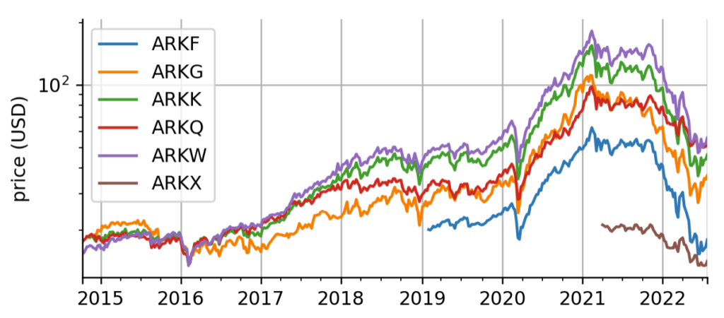
Figure 1: Historical data. Historical weekly, adjusted close prices of the 6 original ARK funds. The y-axis is logarithmically scaled for better comparison.
Probabilistic regime-switching model
Next, we introduce the regime-switching model that we will use to derive the probabilistic Sharpe ratio. We use a hierarchical modeling approach similar to stochastic volatility models in which we describe weekly log-returns as normally distributed values, but both the mean and standard deviation of this Normal distribution are allowed to change over time. To infer the time-varying expected return (the mean of the Normal distribution) and the time-varying volatility (the standard deviation of the Normal distribution) from the short series of returns that we will look at in this example, we use the probabilistic programming framework bayesloop. In probabilistic programming, variables represent random variables that are connected to each other via code, building complex hierarchical models that can then be fitted to data. The Python package bayesloop is a specialized framework that describes times series by a simple likelihood such as a Normal distribution, a Poisson distribution, etc…, but allows the parameters of this likelihood to change over time in different ways.
During inference, we employ Bayesian updating to obtain a new updated parameter posterior distribution after looking at each new data point. However, instead of directly using the previous posterior as the new prior distribution of the next time step, we transform it according to the way that we think the parameters may change from time step to time step (see the animation below). This process is employed in the forward- and backward-direction of time. The combined forward- and backward-pass result in one parameter distribution for each time step that takes into account all other data points. A detailed description of this method can be found in Mark et al. (2018).
Figure 2: Illustration of Bayesian inference for time-varying parameter models. For each point in time we combine the prior distribution (blue) with the likelihood (green) specified by the current data point to obtain the posterior distribution (red). Instead of using the posterior directly as the new prior in the next time step, we transform it according to the hypothesized parameter evolution. The transformed posterior is then used as the new prior.
One example of dynamically changing parameters is the regime-switching model that we will use here. If we "elevate" the posterior distribution a bit between time steps, we assume that there is a small probability that even parameter values far from the current ones might become plausible in the next time step. Using this transformation in the inference process will produce parameter values that jump from time to time. A different example would be slowly drifting parameter values. This can be implemented by blurring the parameter posterior between time steps, assuming that parameter values close to the currently most plausible ones will become likely in the next time step.
Below, you can see a summary of the hierarchical inference process. One advantage of bayesloop is that it uses discrete parameter grids for computing parameter probabilities, allowing for an efficient approximation of the model evidence (also called marginal likelihood). The model evidence can be used to objectively select between different choices for both the likelihood (the low-level model) and different transformations (i.e. different hypotheses about how the parameters change over time; the high-level model).
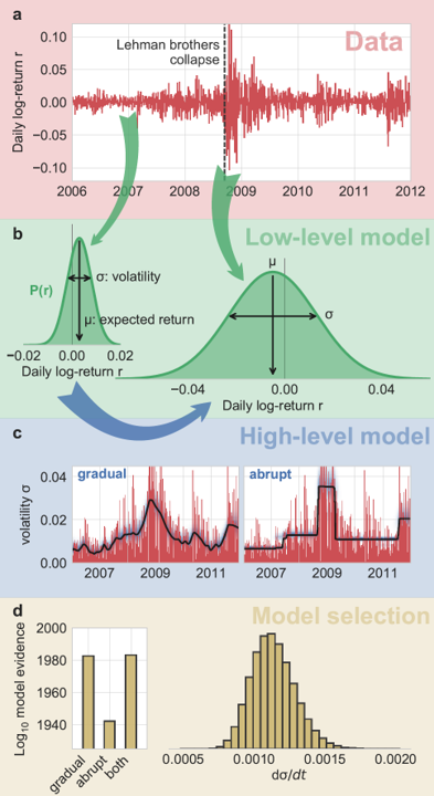
Figure 3: Schematic illustration of the hierarchical modeling approach. Time series data (a) is locally described by a probability distribution with a set of parameters, the low-level model (b). These parameters are allowed to change over longer time scales according to one or more transformations, the high-level models (c). Different hypotheses about the high-level models (i.e. different types of parameter dynamics) can be tested by computing the Bayesian model evidence (d).
Let us look at a single ETF to illustrate the regime-switching model. Here, we pick ARK's flagship fund: ARK Innovation ETF (ARKK). We will evaluate its performance since its inception in 2014. Before we get to the modeling part, we do some further data preprocessing to get the weekly log-returns of ARKK.
Let us look at a single ETF to illustrate the regime-switching model. Here, we pick ARK's flagship fund: ARK Innovation ETF (ARKK). We will evaluate its performance since its inception in 2014. Before we get to the modeling part, we do some further data preprocessing to get the weekly *log-*returns of ARKK. Remember that a log-return is defined as the logarithm of the ratio between subsequent close prices :
Log-returns have the advantage of symmetry, i.e. if on one day the index loses and the next day the index gains , the index attains the original price again. With percentage returns, first losing 10% and then gaining 10% again does not get you back to the original price. Below we plot the cumulative log-returns, that means the logarithmic profit-and-loss one would obtain from buying and holding ARKK from its inception.
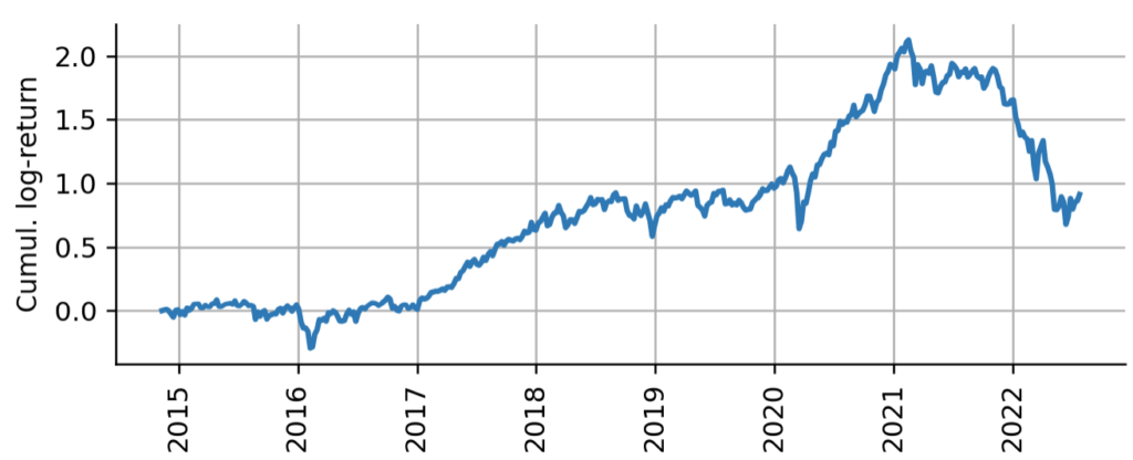
Figure 4: Cumulative log-returns of ARKK. Cumulative weekly log-returns indicate the profit-and-loss one would attain from buying and holding ARKK from its inception, on a logarithmic scale.
The following code below defines the regime-switching model. In bayesloop, all the model specification and data belongs to a Study object, in this case an instance of the HyperStudy class, as we will also infer hyper-parameters that are related to the parameter dynamics. After defining S as our study object, we define the low-level model L, i.e. the distribution from which the observed data points have been drawn. Here, we choose a Gaussian model, fully aware that the Gaussian distribution will only describe the data locally in time, and its parameters will have to change over longer time scales to describe the statistical properties of financial return series such as heavy tails. Note that since bayesloop computes probability (density) values on a regular grid, we need to specify parameter boundaries and grid spacings using closed intervals (bl.cint) or open intervals (bl.oint). This certainly represents a downside of using bayesloop compared to inference algorithms based on sampling techniques, as we have to take care that the boundaries that we set actually provide enough range for the posterior distributions, before actually knowing the posterior distributions. We further specify a non-informative prior in the two parameters mu (expected return) and sigma (volatility).
To enable our two parameters to change over time, we next define the high-level model T using the RegimeSwitch class. Between time steps, this high-level model "elevates" very small probability density values on the parameter grid to the value 10**q, where q denotes the single hyper-parameter of our model. Since we do not know a suitable a-priori value for q, we simply allow a set of discrete values between -4 and 4 with equal prior probability. bayesloop will then infer the posterior distribution of q, employing Occam's razor to allow as many parameter jumps as necessary, but as few as possible to arrive at a parsimonious description of the data.
After setting the low- and high-level model using the S.set method and loading the log-return values with S.load, we call S.fit to start the inference process. bayesloop uses a forward- and backward-pass algorithm similar to the Viterbi algorithm to carry out inference time step by time step, effectively breaking down a very high-dimensional inference problem into many low-dimensional ones. This is bayesloop's niche: Due to the grid-based representation, the number of parameters in the low-level model is restricted to 2-3 in most cases, but these parameters can change over time in both deterministic and stochastic ways. The resulting latent-variable model is very high-dimensional (number of low-level parameter times number of time steps, plus number of hyper-parameters), but by breaking the inference process down along the time axis, bayesloop usually beats other probabilistic programming frameworks within its niche when it comes to computational time.
An additional advantage of this approach that we will not discuss here in detail is the approximation of the marginal likelihood, or model evidence. For each fit, bayesloop provides an absolute value of the model evidence, obtained from integrating over the discrete parameter grids. This provides an easy way to compare models of varying complexity, e.g. a model with static parameters vs. a regime-switching model vs. a model with gradually varying parameters. See the bayesloop documentation for tutorials and examples, or read up on possible applications in cancer research, climate research, policy making, and finance in Mark et al. (2018).
After fitting the model to our series of ARKK returns, we visualize the parameter evolutions. As we can see, ARKK had a slightly positive expected return and a rather stable volatility level up to week #275, which denotes the Corona crash in March 2020. After a sharp decline that is accompanied by a volatility spike, ARKK showed an increased expected return with slightly increased volatility during the Corona-recovery rally of 2020, before the its expected returns turned negative with an even larger volatility about a year after the Corona crash. In the third subplot, you can see the posterior distribution of our hyper-parameter q that tunes the likeliness of parameter jumps.
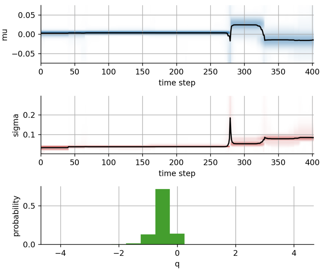
Figure 5: Inferred parameter distributions based on the regime-switching model. The temporal evolution of the expected return mu is displayed in the top panel, the black line indicates the posterior mean value, the shading indicates the uncertainty of the parameter estimate. The temporal evolution of volatility sigma is displayed in the center panel. The bottom panel shows the distribution of the hyper-parameter q, which indicates the likeliness of abrupt parameter jumps.
Robust Sharpe ratio
The regime-switching model fitted above provides us with a joint distribution of expected return and volatility for each trading week. Based on these distributions, we now devise a "robust" Sharpe ratio. For simplicity, we assume a risk-free rate of zero and thus reduce the Sharpe ratio to the signal-to-noise ratio known from physics and engineering:
where denotes the annualized expected return and denotes the annualized volatility. The "classic" Sharpe ratio is thus a point estimate derived from the sample mean and sample standard deviation:
with weekly returns . Below, we demonstrate how we can use the parameter distributions obtained by bayesloop to compute , i.e. the distribution of the Sharpe ratio either averaging over time, taking into account all the different market regimes that the asset has encountered so far, or just taking into account the current regime. We will discuss the latter case in one of the next sections and stick with the time-averaged Sharpe distribution for now. Based on , we can finally compute a "robust" Sharpe ratio by picking a lower percentile on the left tail of . Because will be broader if only few data points (a short track record) are available, picking a point on the left tail will automatically lead to a conservative Sharpe measure that requires a certain track record length to attain a positive value. In the next examples, we will pick first quartile, i.e. we define the robust Sharpe ration as the value that we are 75% certain of achieving.
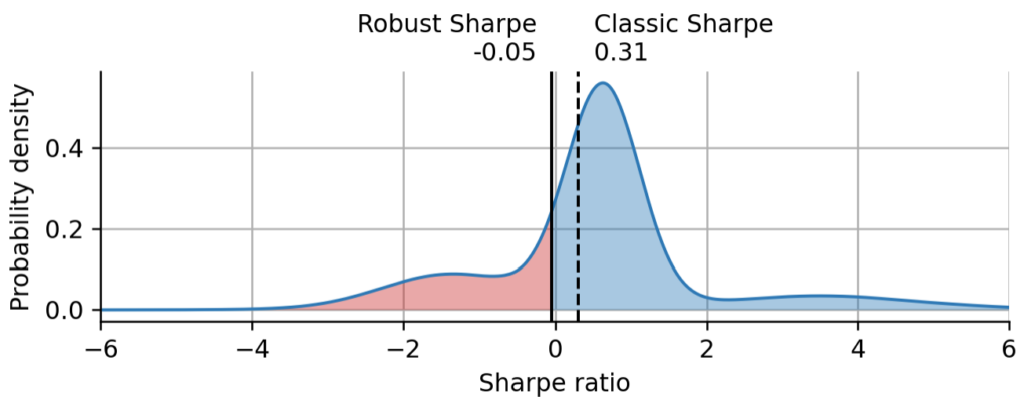
***Figure 6: Sharpe distribution and point estimates. *The blue line and shading shows the distribution of the Sharpe ratio as inferred by the probabilistic regime-switching model. The solid black line marks the robust Sharpe estimate (the first quartile of the Sharpe distribution). The dashed black line marks the classic Sharpe estimate.
Above, we have plotted the Sharpe distribution that we have obtained from the probabilistic regime-switching model, together with the robust Sharpe and the classic Sharpe point estimates. The red shading shows the probability density of the left tail corresponding to our chosen confidence level. We can learn quite a few things from this graph: Even with ~8 years of historical weekly returns, the Sharpe distribution is still very broad, especially since we accounted for regime switches. The Sharpe distribution is not a unimodal bell-shaped distribution, but rather shows a superposition of peaks that correspond to the different regimes/combinations of expected return and volatility. The height of the peaks reflects the fraction of time that the asset has spent in the corresponding regime. As expected, the robust Sharpe is more conservative than the classic Sharpe and at the confidence level of 75%, we cannot assume that ARKK even has a positive Sharpe.
It is interesting to have a closer look at where the classic Sharpe estimate resides within the Sharpe distribution. Because of the multimodal nature of the distribution, the classic estimate does not correspond to a special feature of the distribution, and is lower than the most probable Sharpe ratio according to the Sharpe distribution: .
The most probable Sharpe value (or maximum a posteriori estimate) can be interpreted as follows: this is the Sharpe value that ARKK attains whenever it is in the regime that it spent most of its time in in the past. This can of course be a misleading metric, as there is no guarantee how much time it will spend in this regime in the future. At that point one needs to add expert knowledge about the asset, to hypothesize whether this regime will return. The Sharpe distribution may thus help a fund manager to evoke the right questions to ask about a certain asset and can help to connect past real-world events (e.g. a change in the management of an asset) to quantitative changes in performance. Being able to interpret the different regimes may allow the analyst to have a educated guess about future performance conditional on certain regimes returning and others not.
Finally, we note that we can also measure performance in a slightly different way: rather than reducing the Sharpe distribution to point estimate as we did above, we may ask what the probability is that the Sharpe exceeds a certain threshold value. This approach is along the line of the work of David H. Bailey and Marcos López de Prado (see here, PDF). For example, we can calculate that the probability that the true Sharpe ratio is larger than 1 equals 27.7%. Note that for short track records and skewed or multi-modal distributions, asking for may be much more robust than asking whether !
Estimating performance at the all-time high
To see the value of the robust Sharpe estimate versus the classic estimate, let us assume that today is Feb 15th, 2021, at which we today know with hindsight was the all-time high of ARKK. Let us repeat the inference process, but include only data up to this point, and then again compute the robust Sharpe ratio and the classic Sharpe ratio.
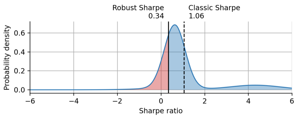
***Figure 7: Sharpe distribution and point estimates at the all-time high of ARKK. *The blue line and shading shows the distribution of the Sharpe ratio as inferred by the probabilistic regime-switching model. The solid black line marks the robust Sharpe estimate (the first quartile of the Sharpe distribution). The dashed black line marks the classic Sharpe estimate.
As expected, both the classic Sharpe estimate and the robust estimate increased compared to the estimates that consider all data, including the recent substantial price decline. However, we can also see that that the classic Sharpe moved almost twice as far compared to the robust estimate. The classic Sharpe estimate is much less conservative compared to the probabilistic model. Even if it certainly depends on the chosen confidence level, but it is still worth noting that the robust Sharpe estimate at the all-time high is very close to the classic Sharpe estimate taking into account all data. This further underlines how the robust Sharpe estimate protects against overestimating Sharpe during or at the end of a price rally.
If we directly compare the two Sharpe distributions, the one considering all data, and the one considering the data only up to the all-time high, we can see that the most probable Share value does not change at all, because it is determined by the earliest regime of ARKK that started with its inception. However, we can see that the regime corresponding to the recent decline is still missing and the right tail is thicker because the data is perfectly timed at the all-time high.
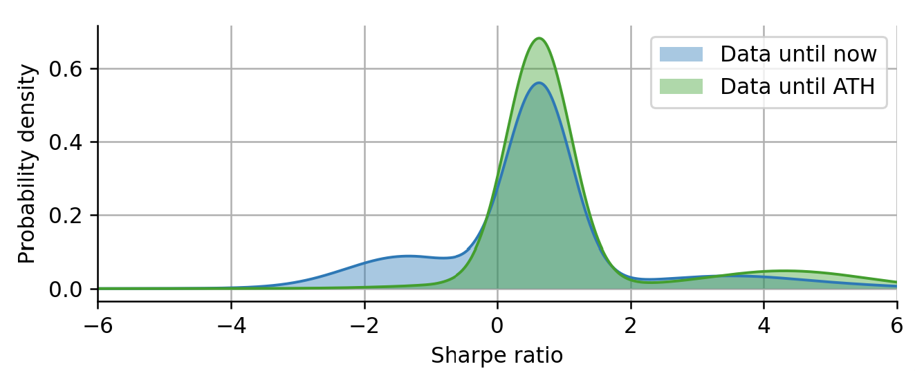
Figure 8: Comparison of Sharpe distribution using all data vs. using data up to the all-time high.
Forget about the past, what about now?
The Sharpe distributions we have discussed so far are all based on the time-average of the posterior distributions, such that each regime contributes to the overall distribution proportionally to the time spent in that regime. However, we may also be interested in just the latest Sharpe distribution, without any time-averaging, for example as the basis of a dynamic allocation of funds to different assets based on various metrics of the latest Sharpe distribution (Sites like Reddit often use an analogue of our robust Sharpe ratio to derive the ordering of popular posts; they also pick a conservative point on the left tail of the "popularity distribution" to penalize posts with high up/down-vote ratio but only few votes in total, see here).
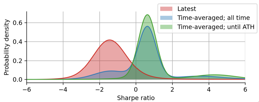
***Figure 9: Latest Sharpe distribution vs. time-averaged Sharpe distributions. *The blue and the green distributions are obtained by averaging the parameter distributions of the regime-switching model over time, whereas the red distribution only takes into account the latest parameter estimates without any time-averaging.
Above we show the time-averaged Sharpe distributions that we have discussed above, and the latest Sharpe distribution for comparison. In contrast to the time-averaged distributions, the latest Sharpe distribution is (usually) not multi-modal, because the asset spends most of its time in only a single regime. Note however that sometimes there is some ambiguity between different combinations of expected return and volatility, so that even the latest Sharpe distribution may occasionally be multi-modal. Even though the latest Sharpe distribution is most often dominated by a single combination of expected return and volatility, it will still exhibit heavy tails because of the uncertainty in the estimation of the expected return and volatility. This is another advantage of the probabilistic, Bayesian approach: estimation errors are seamlessly carried on from the parameters to the final metric that we derive from the Sharpe distribution - such as the robust Sharpe estimate.
bayesloop can carry out the estimation of the latest Sharpe ratio in an online manner, without repeating the full analysis every time a new return value becomes available. For a complete example of such a real-time analysis, see this example from the bayesloop documentation.
Comparing assets with different track record length
Finally, we want to take a look at the Sharpe distributions of all 6 ARK funds. Using the group of ARK funds as an example here is certainly not optimal, as all the returns of these ETFs are highly correlated with each other, even though the individual funds are supposed to have different investment focus. However, we will still uncover some subtle differences in the Sharpe distributions that are of relevance to investors and we can have a closer look at how the length of the track record influences the Sharpe distribution. Below, we first analyze all 6 assets using the model introduced in detail above, and plot the classic Sharpe ratio against the robust Sharpe ratio for a direct comparison.
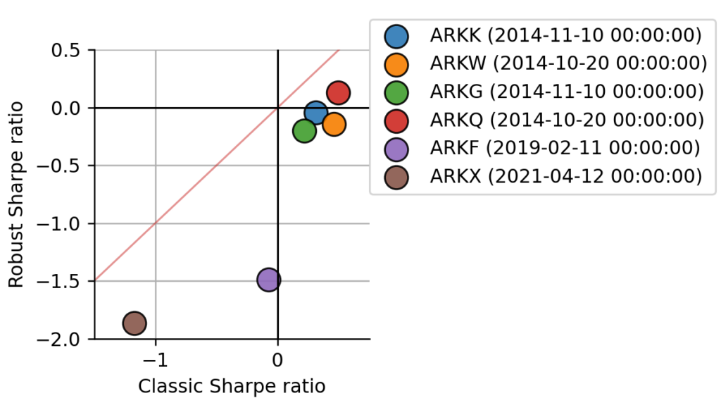
Figure 10: Direct comparison of classic Sharpe estimate and robust Sharpe estimate. Each dot represents one ARK fund. The red line indicates identity line.
The first thing we notice is that the robust Sharpe ratio on the y-axis is always below the classic Sharpe ratio on the x-axis (below the red identity line), as expected, because we choose a conservative confidence level of 75% as before. We also notice that two ETFs attain a much lower robust Sharpe ratio than the others. ARKF and ARKX were issued only in 2019 and 2021, respectively, and this shorter track record is penalized by the robust Sharpe estimate. The difference is best visible in ARKF, which attains a classic Sharpe near zero, still fairly close to the leading group of four, but regarding the robust Sharpe ratio, it is far behind. It is curious, though, that the robust Sharpe values of the two are closer together than their classic Sharpe values. Let us have a closer look at their Sharpe distributions to understand this.
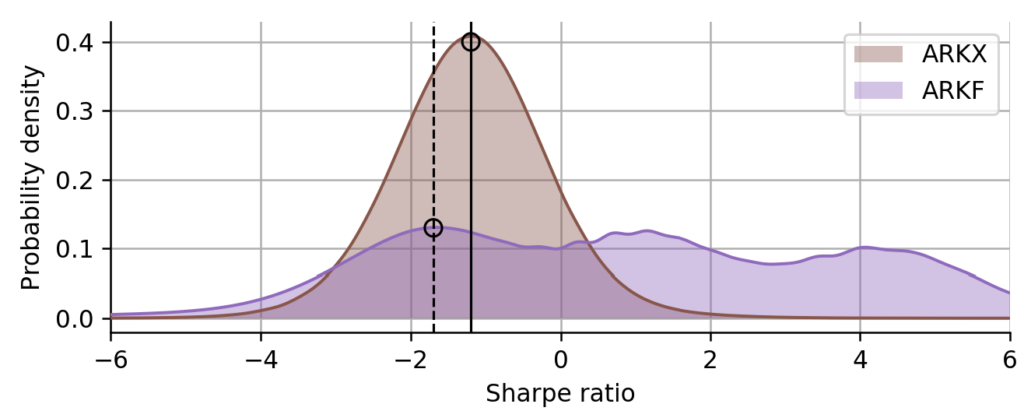
Figure 11: Interpretation of a multi-modal Sharpe distribution. The Sharpe distribution of ARKX is unimodal (brown shading), the most probable Sharpe value is indicated by the solid black line. The Sharpe distribution of ARKF (violet shading) is multi-modal and much broader. However, the left-most peak of the distribution indicates a worse performance of ARKF compared to ARKX in the market regime corresponding to that regime. The most probable Sharpe value in that market regime is indicated by the dashed line.
From their Sharpe distributions, we a few insights into the market conditions that the two funds have seen: being issued in 2019, ARKF has spent almost equal amounts of time in three different regimes, a highly profitable one, a slightly profitable one, and a declining one. ARKX, being issued in April 2021, has only seen the declining regime. However, looking at the left-most peak of the Sharpe distribution of ARKF (dashed line), and comparing it to the peak of the Sharpe distribution of ARKX (solid line), we can conclude that ARKF attains a worse Sharpe ratio in a declining market compared to ARKX. If we now compute the robust Sharpe estimate on the left tail of the distributions, we get quite similar values because ARKF is more spread out in total and stretches towards the left a bit more than ARKX. ARKF with its extremely wide Sharpe distribution is a prime example of how the classic Sharpe ratio can be misleading: the classic Sharpe measures the average variability of the returns by accounting for volatility, but it does not account for the variability in volatility itself.
We can get further insights into the group of 4 funds that are leading the group, also by looking at the difference in the shape of their Sharpe distribution. In particular, we will look at ARKQ, the only ETF that attains a positive robust Sharpe ratio, and at ARKK and ARKW, for which the order is different depending on whether we look at them through the lens of the classic Sharpe ratio or the robust Sharpe ratio. First, we might ask why ARKQ is superior to the other funds. Looking at the Sharpe distributions plotted below, we notice that ARKQ attains the distribution with the thinnest tails, meaning that its regime switches are not as drastic as for example in ARKK or ARKW. There is still some negative skewness in the Sharpe distribution of ARKQ, but among all the ARK funds, it is the one that shows the most consistent positive performance across different market conditions.
We can further deduce from the Sharpe distributions why ARKW attains a slightly larger classic Sharpe ratio compared to ARKK, but a slightly lower robust Sharpe ratio: ARKW shows a more smooth transition between regimes, resulting in a uni-modal but very broad Sharpe distribution. Compared to ARKK, it has a heavier right tail, but also a slightly heavier left tail. Since the robust Sharpe ratio focuses on the left tail, ARKW gets penalized slightly more compared to ARKK. The classic Sharpe ratio rather focuses on the mean of the Sharpe distribution, and in that regard, ARKW is better than ARKK.
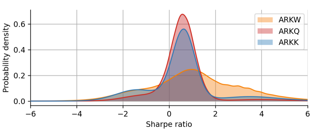
Figure 12: Shape analysis of the Sharpe distribution. Overlay plot of the Sharpe distribution of three different ARK funds that display qualitatively different shapes.
This concludes our analysis of the probabilistic extension of the Sharpe ratio as a performance metric. It is worth noting that other common performance metrics such as the Sortino ratio can be extended in the same manner. For the sake of brevity, we have only looked at one type of parameter evolution, namely the regime-switching model. One can easily add further components to this model, for example to account for a deterministic trend or gradual stochastic fluctuations that allow for an extrapolation beyond the latest Sharpe distribution. Finally, we have not touched another issue with real-world data: bayesloop can easily handle incomplete or missing data. By simply leaving nan values whenever a return value is missing, the inference engine will automatically interpolate the parameter evolution according to the assumptions set by the high-level model.
If you are interested in probabilistic programming in general, stay tuned for our new interactive course that will be offered shortly by Artifact Research!
Get notified about new blog posts and free content by following me on Twitter @christophmark_ or by subscribing to our newsletter at Artifact Research!
Related posts
Probabilistic alpha and beta: quantifying an uncertain edge
In finance, the performance of an asset is often quantified by alpha (the excess returns above a benchmark return) and beta (the volatility or risk of the asset relative to a benchmark). These metrics are estimated from historical data and are often based on only short track records. Even if a long series of historical returns is available for an asset, older data may no longer represent the current market dynamics due to regime switches. In this post, we develop time-varying, probabilistic versions of alpha and beta, and go through the process of using these new metrics to build a dynamic stocks/bonds portfolio to improve on the classic 60/40 portfolio. To accomplish this, we employ probabilistic programming, a technique to build probabilistic models with ease in Python and infer parameters from noisy data.
Skewness: the fallacy of the expected return
In this post we will take a closer look at the expected return that is often stated for investments like stocks and other financial assets, or for certain outcomes in gambling. The point we want to convey is that the expected return is only valid for one period or a single “iteration” (say, one year, or one round of a game such as Blackjack), but that the expected return can be highly misleading for more long-term investments that involve continuous re-investing, i.e. compound interest. We will see that compounding introduces substantial positive skewness in the long-term return distribution. While this skewness certainly represents a beautiful property for building wealth in the long-term, it also renders the expected long-term return misleading as there is a high probability that one will not achieve the long-term expected return! We will learn that to correct for skewness, we need to use the geometric mean instead of the arithmetic mean that is used to compute the expected return – which will lead us to the Compound Annual Growth Rate (CAGR).
How heavy tails destabilize Markowitz portfolio selection
This is the forth and final post of a short series of posts on extreme events in financial time series. In the first post , we have introduced power-law theory to describe and extrapolate the chance of extreme price movements of the S&P500 index. In the second post , we took a closer look at how statistical moments may become infinite in the presence of power-law tails, rendering common estimators useless. In the third post , we have seen how infinite kurtosis makes GARCH risk models fail on out-of-sample data. In this post, we turn to Markowitz’s Modern Portfolio Theory and show how the heavy tails of financial return distributions drastically increase the uncertainty in portfolio allocation weights.