This is the first post of a short series of posts on extreme events in financial time series. We will investigate the return distribution of financial assets, use power-law theory to describe its tails, see how estimating higher moments such as kurtosis becomes meaningless, and finally discuss a fundamental flaw in popular models such as GARCH that arises from fat tails. The point that I want to convey is that without putting much care into the fat-tailedness of financial distributions, models cannot be expected to work out-of-sample, they will always be surprised when that one new extreme data point comes – and those surprises are seldom good ones.
You can access an interactive Python version of this blog post here. It is powered by JupyterLite and runs directly in your browser without any install or config!
Fat tails and Black Mondays
First, we take a look at the distribution of daily returns of the S&P500 index, starting in 1950. This historical series of daily prices contains ~18000 trading days. Rather than looking at prices directly, we will look at the daily log-returns of the S&P500 index. Remember that a log-return $r_t$ is defined as the logarithm of the ratio between subsequent close prices $p_t$:
$$r_t = \log(\frac{p_t}{p_{t-1}})$$
Log-returns have the advantage of symmetry, i.e. if on one day the index loses $r_t = -0.1$ and the next day the index gains $r_{t+1} = +0.1$, the index attains the original price again. With percentage returns, first losing 10% and then gaining 10% again does not get you back to the original price.
We find that the worst day-to-day log-return was -0.229, corresponding to an arithmetic return of -20.5%, and that it happened on Monday, October 19, 1987 – the so-called Black Monday. To put this Black Monday into proper context, we plot the sample distribution of daily log-returns, showing us how frequent we observe daily returns of a certain sign and magnitude. Note that we set a logarithmic scaling for the y-axis to get a better view on the tails of the distribution, i.e. the very large but rare negative and positive returns – the crashes and the rallies:
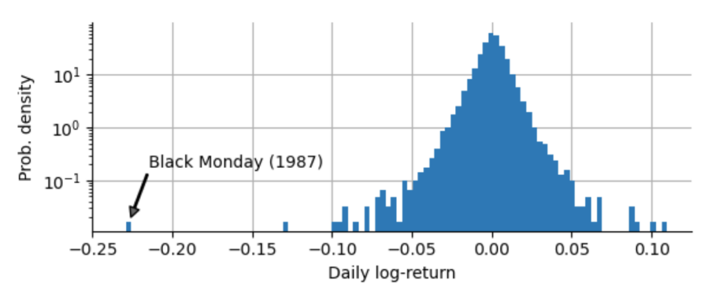
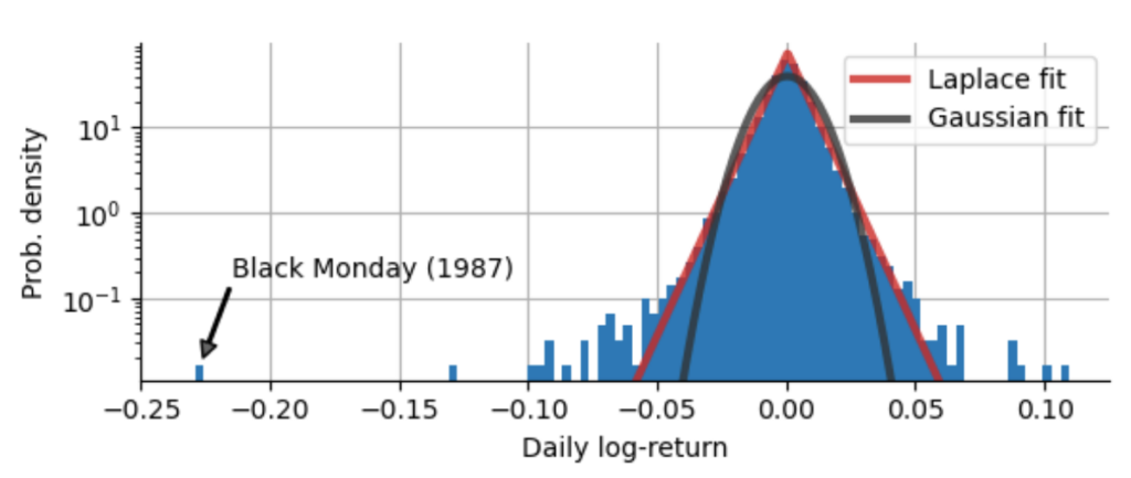
How can we describe the decay of the distribution of returns? With the logarithmic scaling of the y-axis, an exponential decay appears as a linear decay, so we might suspect that for small absolute returns, the distribution decays exponentially, but as the absolute returns grow larger, we deviate more and more from the initial slope. Actually, we can show that neither the ubiquitous Gaussian distribution (also called Normal distribution), nor the Laplace distribution with its exponential decay on both sides accurately model the return distribution of the S&P500. Both the Gaussian distribution and the Laplace distribution underestimate the probability of extreme events, of rallies and crashes:
Counting sigmas
As we can see above, both the Gaussian distribution and the Laplace distribution drastically underestimate the chance of very strong market movements! Often you might read something about “that was a 3-sigma market move” or the like, because many people like to compare individual returns to the standard deviation (called “sigma”) of a fitted Gaussian distribution. However, if the Gaussian distribution does not fit the sample distribution at all like in our case, measuring a crash in units of “sigma” can be highly misleading! To show this, we first check by how many sigmas the market moved on the Black Monday of 1987, by dividing the absolute log-return of the Black Monday by the standard deviation of our log-return distribution:
$$\frac{0.2290}{0.0099} = 23$$
Based on the Gaussian distribution, the Black Monday would be a “23-sigma” event! Now, the Gaussian distribution clearly tells us how often an X-sigma event should occur:
- 1-sigma: approx. 1 out of 3 days
- 2-sigma: approx. 1 out of 22 days
- 3-sigma: approx. 1 out of 370 days
- …
- 23-sigma: approx 1 out of 10$^{\text{116}}$ days
Let’s be clear here: Based on a Gaussian distribution, the daily loss of the Black Friday in 1987 should be a event that we expect to happen once every 10$^{\text{116}}$ days. This number is pretty much incomprehensibly large. If the S&P500 started trading right after the birth of the universe, that would have been only 10$^{\text{13}}$ trading days. After 10$^{\text{116}}$ days, all stars in the universe will long be burnt out, even all black holes will have evaporated and the universe will be a dark and empty place. So either we should be very happy to have that one expected Black Friday in the history and future of the universe behind us already, or you really should never ever use a Gaussian distribution to model stock returns! Regardless of the market and the details, if someone talks about 10-sigma events or 23-sigma events, they are using the wrong model for sure, as the chance of observing such an event in our lifetime is minuscule.
So the question is: How do we treat such extreme data points? Should we mark them as outliers or artifacts, to make our financial models conform better to the majority of data points? Certainly not, since the outcome of our investing may critically depend not on the majority of smaller returns, but especially on such extreme events! In the following paragraphs, we get to know an approach that can account for and extrapolate beyond extreme events like the Black Monday.
Power-law statistics
Now that we know that the Gaussian distribution is not a good choice, what type of distribution can in fact describe the frequency of extreme events that shake up the S&P500? The frequency of extreme positive returns and extreme negative returns is not equal for most financial assets, as crashes generally are more self-reinforcing than rallies. That is why we will focus on the left (negative) tail of the return distribution in the following.
Since we are only interested in the extreme events, we will only consider returns that are smaller than -0.03 (about three standard deviations from the mean). Below, we visualize these extreme negative returns on a log-log scale (we use the absolute value of the negative returns here). Both the y-axis (which shows how often a log-return of a given magnitude occur) and the x-axis (which shows the magnitude of the log-return) are scaled logarithmically:
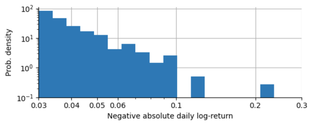
As we can see, this histogram of extreme absolute returns falls off approximately linearly in a log-log-scaling. Whenever you spot a straight line in a log-log-plot, this indicates a so-called power-law. The power-law relation of the probability of observing a large absolute log-return is given as:
$$p(|r_t|) = c \cdot |r_t|^{-\alpha}$$
The constant $c$ does not bother us too much at this moment, it simply ensures that the left side of the equation is properly normalized, but the exponent $\alpha$ is very interesting as it tells us how the power-law works. If you know the frequency of a given absolute log-return, then the power-law will tell you how many times less probable a log-return of double the size would be:
$$p(2 \cdot |r_t|) = c \cdot (2 \cdot |r_t|)^{-\alpha} = 2^{-\alpha} \cdot c \cdot |r_t|^{-\alpha} = 2^{-\alpha} \cdot p(|r_t|)$$
or simpler:
$$\frac{p(2 \cdot |r_t|)}{p(|r_t|)} = \frac{1}{2^{\alpha}}$$
For $\alpha=0$, all returns are equally probable, for $\alpha=2$, doubling the return makes it 4-times less likely to occur. Since this rule for doubling up or down does not depend on the value of $|r_t|$ itself but works for all values of $|r_t|$, power-law relations are also called “scale-free” or scale invariant.
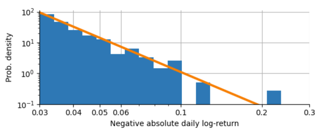
What about the exponent $\alpha$ for our extreme negative S&P500 log-returns? We can easily estimate it from the data, but there are some subtleties about the correct binning of the histogram above that may bias our estimate (see e.g. White et al. (2008)). To circumvent these binning issues, we can instead estimate the power-law exponent of the cumulative histogram of log-returns and then subtract one from the obtained slope:
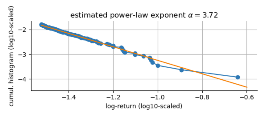
From this estimation, we obtain a power-law exponent of $\alpha \approx 3.7$. If we plot the original histogram of our extreme negative log-returns, we can see that it nicely captures the decline in likelihood as the crashes grow larger in magnitude. However, this power-law exponent still underestimates the probability of another Black Monday happening, as the fit line does not perfectly hit this extreme point. If we would want to create an even more conservative model of extreme events, we would need to manually decrease the value of $\alpha$ further to account for a larger probability of Black Mondays happening, at the expense of losing fit accuracy for the smaller crashes. This is the first time that we can see how a single data point affects our modeling decisions. For now, we will trust the parameter estimation and go along with the estimate $\alpha=3.7$.
We can use this power-law to extrapolate how often we would expect a Black Monday (or “23-sigma event”) to occur in the long run. From the data we have, we can estimate that the chance of observing a decline of -0.03 or worse is about 1.6%. Following our power-law curve, the Black Monday decline of -0.229 would thus occur $\left(\frac{0.229}{0.03}\right)^{-3.7} \approx \frac{1}{1845}$ as often as a -0.03 decline that we observe about once every three months. This means that based on our power-law curve, Black Mondays like the one in 1987 are expected to happen about once every 450 years.
If we included more data that contain other examples of extreme events, e.g. from the Great Depression, this estimate could become even smaller. Likewise, if we would adjust the power-law exponent to be more conservative than our simple estimation method suggests, we would also get a shorter period. While 450 years still is a very long period, it is a much more realistic estimate compared to the 10$^{\text{114}}$ years we got using the Gaussian distribution. One advantage of the power-law model is its power to extrapolate: using the estimate of the power-law exponent 𝛼 and the frequency of smaller returns on which we have good data, we can estimate the frequency of future severe crashes on which we have not yet obtained any data.
TAKE-HOME MESSAGE

There is no such thing as a "10-sigma event" or even a "23-sigma event"! A true 10-sigma event is so incredibly rare that experiencing it within our lifetimes is minuscule. Extreme events certainly happen, but they cannot be described by "sigmas", they need to be accounted for and extrapolated using power-law theory. Always be careful when analysts excuse themselves for not being prepared for a "10-sigma event", as this indicates that their risk models are utterly flawed.
In the next post, we will make use of our estimated power-law exponent $\alpha$ to have a closer look at the statistical consequences of fat-tailed distributions, in particular we will see that estimating statistical moments such as kurtosis becomes meaningless in certain cases.
The content of this post is part of an interactive course on risk mitigation that is currently under development and will be offered shortly by Artifact Research. Our courses are all based on interactive Python notebooks that run directly in your browser without any install or config. This way you can get a better understanding of abstract relations by tinkering with code and changing parameters of models. A free interactive preview of this post series is available here!
Get notified about new blog posts and free content by following me on Twitter @christophmark_ or by subscribing to our newsletter at Artifact Research.
Very good article. I definitely appreciate this website. Stick with it!