This is the second post of a short series of posts on extreme events in financial time series. In the previous post, we have introduced power-law theory to describe and extrapolate the chance of extreme price movements of the S&P500 index. In this post, we will explore how the power-law tails of a return distribution affect the estimation of metrics such as variance and kurtosis, which lie at the heart of many popular risk models in finance like GARCH and Modern Portfolio Theory. The point I want to convey in this post is that even if you will always estimate a finite sample estimate for kurtosis from a given data set, the true kurtosis that underlies the data generation process (the market) is infinite and many models will fall for the apparent finite sample kurtosis!
You can access an interactive Python version of this blog post here. It is powered by JupyterLite and runs directly in your browser without any install or config!
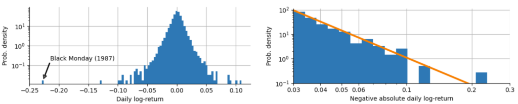
In the previous post “The 23-sigma fallacy” we have investigated the distribution of daily log-returns $r_t$ of the S&P500 index starting in the year 1950 (see below, left graph), and we have shown that the tails of this distribution do not follow a Gaussian or Laplace distribution, but rather that the tails fall off with a power-law relation $p(r_t) \sim |r_t|^{-\alpha}$ (see below, right graph). We estimated the power-law exponent to $\alpha = 3.7$ in the case of the S&P500 data. In this post, we will start to explore the consequences that the value of $\alpha$ entails.
The power-law exponent $\alpha$ actually tells us a lot about the stability and finiteness of the moments of a probability distribution, and that in turn has implications for some of the most commonly employed models in finance. The first four central moments are:
- Mean: The expected value of the distribution
- Variance: The square of the standard deviation, often used to estimate the volatility based on a return distribution
- Skewness: Measures the lopsidedness of a distribution. Return distributions tend to have negative skewness as crashes are more severe than rallies.
- Kurtosis: Measures the heaviness of the tails of the distribution. Return distributions usually have a kurtosis that is larger than that of the Gaussian distribution, i.e. extreme events happen more often than expected in a Gaussian model.
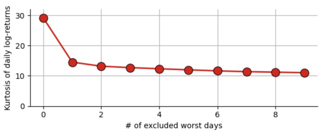
The kurtosis of a Gaussian distribution is equal to 3 (using Pearson’s definition, with Fisher’s definition of the excess kurtosis it is 0), but our sample of daily S&P500 log-returns has a kurtosis of 29.3, indicating again that extreme events are much more likely to happen that we would assume using a Gaussian model. This brings us to the question: How much power does a single data point have on our estimate of kurtosis? If we re-calculate the kurtosis of all daily log-returns of the S&P500 since 1950 and only remove the Black Monday of 1987, we get a value of 14.6, almost half of the value we get when we use all values! Removing further worst days of course further decreases the kurtosis, but the effect is significantly smaller.
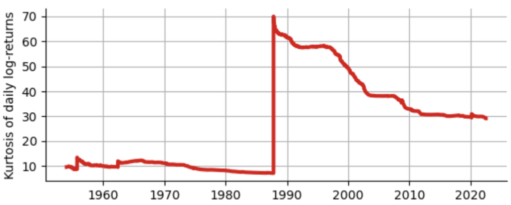
A more drastic view on this problem is gained if we plot kurtosis in a walk-forward manner, i.e. for each day, we plot the estimated kurtosis using all past log-returns up to this point in time. As you can see below, until the Black Monday, kurtosis never exceeds a value of 15, yet even 35 years after the Black Monday, kurtosis has not yet “recovered” from that one event and stays around 30. Does this mean we should just ignore the Black Monday as an outlier and proceed using our “clean” estimate of 14.6? No, definitely not! As we will shortly see, we should rather ask ourselves whether it makes any sense to estimate kurtosis at all!
The fact that one data point can shift our estimate of kurtosis in such a strong way that it does not seem to converge anymore as we add more data points is a clear indication that the kurtosis of the underlying probability distribution is actually infinite! The problem is that for a finite data sample (and all data sets are finite) we will always be able to estimate a finite value of kurtosis. The numerical estimator we use here (from the Python module scipy.stats.kurtosis) cannot return $\infty$, it will always report a finite sample kurtosis. But this finite estimate will not help us to say anything about the future behavior of a market, because kurtosis will keep being shifted to even higher values by another Black Monday, another Black Tuesday, … in the more or less distant future.
However, the power-law description of the frequency of extreme events that we introduced above can help us to decide whether kurtosis is finite, so that after seeing enough data points to estimate the power-law exponent we can decide whether we should accept the fact that kurtosis cannot be estimated and really is infinite. To see that, we need to make use of a special probability distribution, the Student’s t-distribution. It is a bell-shaped symmetric distribution with power-law tails. Its additional parameter $\nu$ defines the power law exponent $\alpha=(\nu+1)$. Below we fit a t-distribution to our S&P500 log-returns, while keeping the power-law exponent of $\alpha=3.7$ (corresponding to $\nu=2.7$) that we have estimated before:
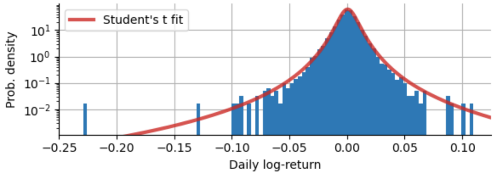
One can certainly question whether the Student’s t-distribution really is a good fit to our log-returns, as it overestimates the frequency medium absolute returns and still underestimates the probability the Black Monday. For the moment, we ignore these details and focus on the kurtosis of the Student’s t-distribution and the relation to the power-law exponent $\alpha$:
- $\text{Kurt} = \frac{6}{\nu-4} + 3~$ for $~\nu > 4~$ or $~\alpha > 5$
- $\text{Kurt} = \infty$ for $~2 < \nu \leq 4~$ or $~3 < \alpha \leq 5$
- otherwise undefined
This confirms our initial guess that with a power-law exponent of $\alpha \approx 3.7$, kurtosis really is infinite and it makes no sense to estimate it from a finite sample, as the estimated value will only hold until the next extreme event that will push it even higher. We can easily simulate this effect by drawing random samples from Student’s t-distributions with different power-law exponents that correspond to the three regimes noted above. Below, we draw 100000 random numbers from t-distributions with $\alpha=2$, $\alpha=3.7$, $\alpha=6$, and then compute kurtosis in a walk-forward manner as before, to see how the estimated sample kurtosis evolves over time in the three different cases:
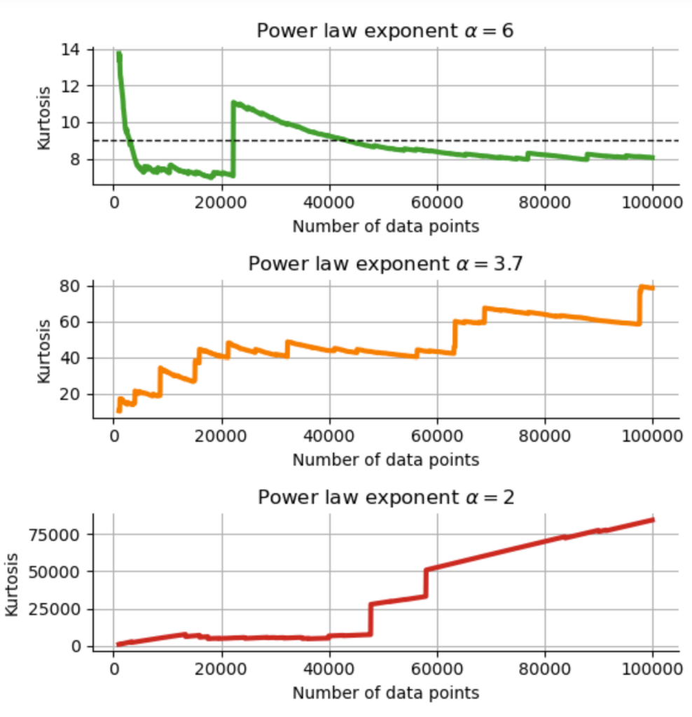
In the case $\alpha=6$ ($\nu=5$), kurtosis is finite and should assume a value of $\frac{6}{\nu – 4} + 3 = 9$. While we do see some fluctuations, the estimated value of kurtosis slowly approaches the true value. For the example that corresponds to the power law exponent of the S&P500 with $\alpha=3.7$, the simulation shows the same behavior as the real data: no convergence can be detected, rather each extreme event pushes kurtosis higher; in the limit of infinite samples, we would reach infinite kurtosis. In the third case with $\alpha=2$, kurtosis of the Student’s t-distribution is not even properly defined, and we can see yet another type of behavior in the simulation: now a majority of data points increases the kurtosis estimate, not just a few individual extreme samples. With such a slowly decreasing power law, extreme values are ubiquitous, pushing kurtosis higher and higher in simulation.
TAKE-HOME MESSAGE

Even if certain properties of probability distributions are infinite, we will always find finite sample estimates when looking at a given data set, simply because the data set contains only a finite number of data points. However, if power law theory clearly tells us that a certain property is infinite, we must not use the finite estimates anywhere and we must not use models that require this property to be finite! If we do it anyway, it will at best only work until the next extreme event, which will invalidate our past estimates and - in the case of financial models - might bankrupt us!
As kurtosis increases – or becomes infinite – it also affects lower moments, most importantly variance. The square root of variance is the standard deviation, or volatility as it is called in the finance. Volatility is an ubiquitous parameter in portfolio optimization and almost every financial model as it ended up being the most commonly used estimator of “risk”. To see how kurtosis affects the estimation of volatility, we conduct a simple Monte Carlo experiment: We draw 50 years of daily returns from a probability distribution of our choice (we’ll use the Gaussian and the Student’s t-distribution), and compute the volatility estimate using the sample standard deviation. We do this not only once, but 10000 times, each time we draw new hypothetical 50 years of daily returns and compute the corresponding volatility estimate. Of course, those estimates will not all be the same but will fluctuate around the true volatility as we only have a finite number of data points. Since we know the true probability distribution that we use for the simulation, we also know the true volatility. To see how accurate we can estimate the volatility based on 50 years of data, we compute the relative error between volatility estimates and the true volatility.
We find the following relative errors for different choices of return distributions:
- Gaussian distribution; rel. error of $\approx 0.5\%$
- Student’s t-distribution with $\alpha=6.0$ ($\nu=5.0$); rel. error of $\approx 1.0\%$
- Student’s t-distribution with $\alpha=4.0$ ($\nu=3.0$); rel. error of $\approx 3.8\%$
- Student’s t-distribution with $\alpha=3.7$ ($\nu=2.7$); rel. error of $\approx 6.1\%$
With a power-law exponent of $\alpha=3.7$ (corresponding to $\nu=2.7$; as we have estimated for the S&P500 to explain the Black Monday), 50 years worth of daily returns still result in an estimation error of volatility of over 6%! Note that this large estimation error will grow even faster as we approach $\alpha=3.0$, because variance becomes infinite for the Student’s t-distribution at $\alpha=3.0$ ($\nu=2.0$). Based on our Student’s t approximation of the S&P500 return distribution the estimation error of volatility increased 12-fold (!) from what we would expect assuming a Gaussian distribution.
TAKE-HOME MESSAGE

The heavier the tails of a return distribution, the more data points are necessary to achieve a required confidence in certain parameter estimates. Remember this every time you try to assess the risk of investing in a relatively new financial asset for which only a few years of data are available.
In the next post, we will further investigate the consequences of infinite kurtosis for the popular GARCH risk model in finance. We will show that GARCH is extremely good a describing the statistical properties of financial time series (including the volatility spikes during crashes), but that it falls for the trap of the finite sample kurtosis – with the consequence that it will always be surprised by the next even larger extreme event instead of anticipating it!
The content of this post is part of an interactive course on risk mitigation that is currently under development and will be offered shortly by Artifact Research. Our courses are all based on interactive Python notebooks that run directly in your browser without any install or config. This way you can get a better understanding of abstract relations by tinkering with code and changing parameters of models. A free interactive preview of this post series is available here!
Get notified about new blog posts and free content by following me on Twitter @christophmark_ or by subscribing to our newsletter at Artifact Research.
2 thoughts on “Infinite kurtosis: moment statistics under fat tails”