Why GARCH models fail out-of-sample
This is the third post of a short series of posts on extreme events in financial time series. In the first post, we have introduced power-law theory to describe and extrapolate the chance of extreme price movements of the S&P500 index. In the second post, we took a closer look at how statistical moments may become infinite in the presence of power-law tails, rendering common estimators useless. In this post, we will investigate the consequences of infinite moments by showing how the popular GARCH risk model almost perfectly describes in-sample data, but fails to extrapolate to out-of-sample data.
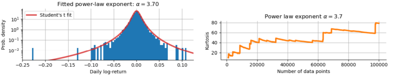
In the previous post "Infinite kurtosis" we have modeled the log-returns rt of the S&P500 index using a Student's t-distribution with a power-law tail exponent of (see below, left). We then continued to show that the kurtosis (the forth statistical moment, measuring the likelihood of extreme values) of a distribution with this power-law exponent is infinite. Importantly, if we estimate the sample kurtosis from historical data, we will always get a finite estimate, but this estimate will not hold in the future and will continue to rise whenever a new extreme return appears in the S&P500 (see below, right). In this post, we will investigate how the popular GARCH risk model is mislead by the finite sample kurtosis fails to extrapolate beyond historical events!
Generalized autoregressive conditional heteroskedasticity (GARCH) models are widely believed to yield accurate descriptions of return distributions as they are able to replicate many of the anomalous properties of sample return distributions by allowing volatility to spike up from time to time - thus emulating the self-enforcing nature of volatility during crashes and rallies. However, we will argue that this ability to accurately describe the statistical properties of any finite data sample is not enough, and that GARCH models will always be surprised by new extreme events because they do not extrapolate beyond what has already been seen. In the simplest GARCH(1,1) model with a constant price trend , log-returns are modeled as
with the variance of the random random fluctuations defined via the following recursion:
Note how the variance (and thus volatility) depends on both the previous variance and the realized log-return. Note also that while the equation above defines the variance of , we may still choose different distributions to draw the values from. The default choice is the Gaussian distribution, but one can also choose a more heavy-tailed distribution such as a Student-t distribution. In Python, GARCH models can be easily implemented using the well-documented arch package. To gain some better intuition on the GARCH(1,1) model, we simulate alternative histories of the S&P500 based on the fitted parameter values of the GARCH(1,1).
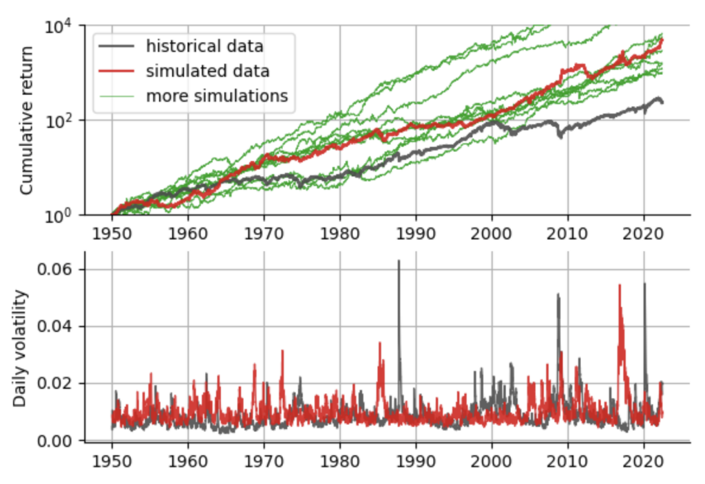
Looking at the simulated data vs. the real historical data, we can learn a few things: the GARCH(1,1) does a pretty good job in modeling volatility spikes, regarding the frequency and magnitude of the spikes and it produces realistic looking equity curves with crashes and rallies. We further notice that all simulations attain a larger cumulative return compared to the real S&P500. The main reason for this overly good performance is that the GARCH(1,1) model as defined here does not allow for asymmetry, whereas it is known that the negative tail of the real return distribution shows more extreme values than the positive tail.
We can improve on this by explicitly adding asymmetry both to the GARCH process itself (resulting in a GJR-GARCH model with the additional parameter ) and also to the distribution that we draw our noise terms from (choosing a Standardized Skewed Student's distribution, see here and here for further info). Again, we can readily fit this model to our data using arch, and then see whether the results now match the true S&P500 more closely:
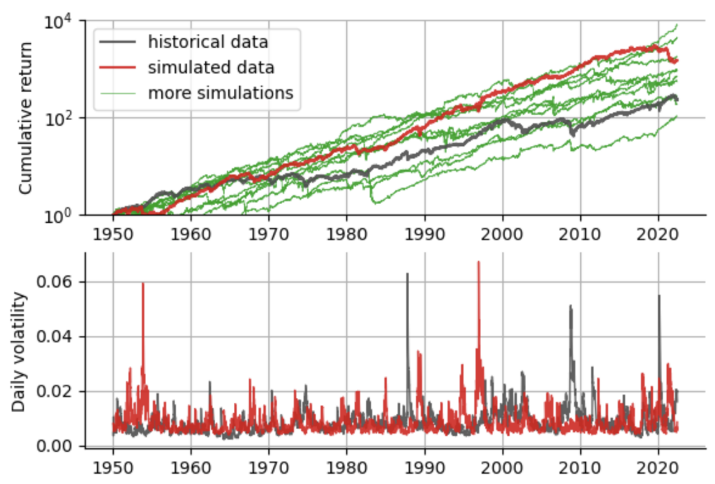
Indeed, when accounting for the asymmetry in the distribution of returns (i.e. crashes have a larger magnitude than rallies on average), we get a better match to the real data. Now that we have some understanding of how the GARCH model works, and we have seen that it does a pretty good job of approximating the past S&P500 data, we can close in on the intricate flaw of the GARCH model. To illustrate this flaw, we again turn to higher moments of the return distribution, namely to kurtosis. The problem is that GARCH's greatest strength - namely to accurately model almost all statistical properties of the data at hand - is also it's biggest weakness when it comes to the fat tails of financial time series.
In the previous blog post of this short series, we have seen that the kurtosis of a distribution with power-law tails and a power-law exponent of (fitted to the S&P500 returns) is actually infinite. While we can derive this property indirectly from power-law statistics, we will never see an infinite sample kurtosis. All data samples we will ever have are finite, we have a certain number of days/months/years to look back, and thus we can always estimate the sample kurtosis and get some finite value. And GARCH falls for this: it sees the finite sample kurtosis value of the data at hand, and then replicates this value, instead of extrapolating like the power-law model. This focus of GARCH on the seen data rather than on the yet unseen data that might come in the future thus will lead to an underestimation of the magnitude of future crashes. Of course, after the next bigger-than-ever crash, sample kurtosis will go up and GARCH will follow and accurately model the new sample kurtosis - but only after the damage is done.
We can nicely illustrate this effect by using the simulation feature of the arch package. Again, we fit the real series of S&P500 returns using the basic GARCH(1,1) with Gaussian noise, and the asymmetric GARCH(1,1) with the skewed Student-t noise. For both cases, we then simulate 500 hypothetical years of S&P500 performance. Finally, just like before when we were discussing the stability of higher statistical moments, we compute the sample kurtosis over time, to see how the estimate evolves over time as more and more data from our 500-year simulation becomes available.
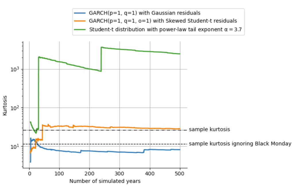
The results we get from this simulation are quite revealing: The kurtosis of the default, symmetric GARCH process stabilizes around the sample kurtosis of the S&P500 returns without accounting for the worst day, the Black Monday of 1987. Since the left tail of the S&P500 return distribution is more extreme than the right tail, fitting a symmetric process will naturally underestimate the probability of extreme events in the left tail and overestimate the probability of extreme events in the right tail. As the Black Monday is in the far left tail and accounts for about half of the sample kurtosis, the symmetric GARCH process ends up replicating the sample kurtosis excluding this data point.
The asymmetric GARCH process can account for the heavier left tail of the return distribution and thus nicely replicates the sample kurtosis of the data. However, both of these GARCH processes fall into the trap of infinite moments: they replicate the finite sample kurtosis when in reality, kurtosis is infinite. In the plot above, we also show the sample kurtosis of a Student-t distribution with the power-law tail exponent of as we have fitted earlier in this lecture. As we can see, the sample kurtosis of the power-law model does not stabilize, but rather climbs higher and higher, up to ~100 times the sample kurtosis of the data within the 500 years that we simulate, clearly indicating that the true value of kurtosis is infinity.
In the next post, we will further investigate the consequences of infinite kurtosis and its destabilizing effect on lower moments, especially on variance and thus on volatility. We will illustrate this effect by showing how Modern Portfolio Theory and the allocation weights for financial assets derived from it suffer under the presence of infinite moments.
The content of this post is part of an interactive course on risk mitigation that is currently under development and will be offered shortly by Artifact Research. Our courses are all based on interactive Python notebooks that run directly in your browser without any install or config. This way you can get a better understanding of abstract relations by tinkering with code and changing parameters of models. A free interactive preview of this post series is available here!
Get notified about new blog posts and free content by following me on Twitter @christophmark_ or by subscribing to our newsletter at Artifact Research.
Related posts
The 23-sigma fallacy
This is the first post of a short series of posts on extreme events in financial time series. We will investigate the return distribution of financial assets, use power-law theory to describe its tails, see how estimating higher moments such as kurtosis becomes meaningless, and finally discuss a fundamental flaw in popular models such as GARCH that arises from fat tails. The point that I want to convey is that without putting much care into the fat-tailedness of financial distributions, models cannot be expected to work out-of-sample, they will always be surprised when that one new extreme data point comes – and those surprises are seldom good ones.
Infinite kurtosis: moment statistics under fat tails
This is the second post of a short series of posts on extreme events in financial time series. In the previous post , we have introduced power-law theory to describe and extrapolate the chance of extreme price movements of the S&P500 index. In this post, we will explore how the power-law tails of a return distribution affect the estimation of metrics such as variance and kurtosis, which lie at the heart of many popular risk models in finance like GARCH and Modern Portfolio Theory. The point I want to convey in this post is that even if you will always estimate a finite sample estimate for kurtosis from a given data set, the true kurtosis that underlies the data generation process (the market) is infinite and many models will fall for the apparent finite sample kurtosis!
How heavy tails destabilize Markowitz portfolio selection
This is the forth and final post of a short series of posts on extreme events in financial time series. In the first post , we have introduced power-law theory to describe and extrapolate the chance of extreme price movements of the S&P500 index. In the second post , we took a closer look at how statistical moments may become infinite in the presence of power-law tails, rendering common estimators useless. In the third post , we have seen how infinite kurtosis makes GARCH risk models fail on out-of-sample data. In this post, we turn to Markowitz’s Modern Portfolio Theory and show how the heavy tails of financial return distributions drastically increase the uncertainty in portfolio allocation weights.