Probabilistic alpha and beta: quantifying an uncertain edge
In finance, the performance of an asset is often quantified by alpha (the excess returns above a benchmark return) and beta (the volatility or risk of the asset relative to a benchmark). These metrics are estimated from historical data and are often based on only short track records. Even if a long series of historical returns is available for an asset, older data may no longer represent the current market dynamics due to regime switches. In this post, we develop time-varying, probabilistic versions of alpha and beta, and go through the process of using these new metrics to build a dynamic stocks/bonds portfolio to improve on the classic 60/40 portfolio. To accomplish this, we employ probabilistic programming, a technique to build probabilistic models with ease in Python and infer parameters from noisy data.
DISCLAIMER: Financial analyses and trading strategies that are presented on this site are not a recommendation to buy or sell, but are for educational purposes only. Neither I personally nor Artifact Research GmbH accepts any liability whatsoever for any loss arising from any use of this information.
Data
In our toy example, we want to invest in the S&P500 via the ETF SPY, and we want to hedge against market crashes by investing in the 20+ years treasury bonds ETF TLT. Note that we will not discuss whether TLT really represents a good hedge against market crashes in this post, we use this pair of assets simply because it is often praised as a stable long-term investment as the 60/40 portfolio.
Below, we load the daily price data from Yahoo Finance for these two assets and compute the weekly log-returns. We further add a column for the risk-free rate. For simplicity, we will set the risk-free rate to zero in our example, but we include the column so that the code below generalizes to more complicated cases. asdasd
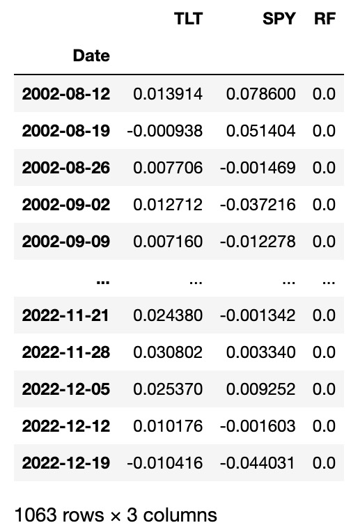
Data table that contains weekly returns of SPY and TLT and forms the basis for the following analyses.
CAPM likelihood function
Next, we need to define alpha and beta. We do this via a Capital Asset Pricing Model (CAPM), in our case also called Single Index Model (SIM). In particular, we model the log-return of TLT as follows:
where denotes the risk-free rate, denotes the return of the market (in our case, the return of SPY), and denotes Gaussian noise. This equation implies some rather unrealistic assumptions. First, it assumes that the asset log-returns (minus the risk-free rate) is linearly related to the market log-returns (minus the risk-free rate), whereas financial assets are known to feature highly non-linear relations. Second, the CAPM model assumes that the random fluctuations follow a Gaussian distribution, even if it is known that financial time series commonly follow heavy-tailed distributions (for which extreme values occur more frequently). Third, the model defined above assumes that and are constant metrics that do not change over time. The performance of many financial assets, however, will depend on macro-economic conditions, product life-cycles, change in management, etc.
Before we will see how to overcome at least some of the issues described above, we turn the formula above into a Python function that specifies the likelihood function for the model defined above. This likelihood function returns the probability (density) of observing a given log-return, given the parameter values for , , , and the additional data points and . This likelihood function can then be used to infer parameter values from data by employing e.g. Maximum Likelihood Estimation or Bayesian inference. We will discuss a special case of Bayesian inference for this model below.
Probabilistic regime-switching model
Next, we introduce the regime-switching model that we will use to turn the and parameter of the CAPM model into time-varying probabilistic parameters. This model is similar to the one used in a previous post on the probabilistic Sharpe ratio. We use a hierarchical modeling approach that assumes the the CAPM model holds locally in time, but that the parameters , , and may change abruptly over longer time scales due to regime switches in market conditions. Turning the parameters of the CAPM model into time-varying parameters (or latent variables) also at least partially alleviates other issues: a dynamically changing will produce a heavy-tailed distribution by a superposition of different Gaussian distributions when averaged over longer periods of time, similar to stochastic volatility models. Moreover, a dynamic and are able to encode non-linear correlations between assets by approximating them locally by a linear correlation. Our model will thus be able to capture essential properties of the data that the original CAPM model fails to recognize. However, the regime-switching model we are about to implement will not attempt to predict market regime-switches, it will only react very fast to them!
To infer the time-varying parameters , , and from the series of returns that we will look at in this example, we use the probabilistic programming framework bayesloop. In probabilistic programming, variables represent random variables that are connected to each other via code, building complex hierarchical models that can then be fitted to data. The Python package bayesloop is a specialized framework that describes times series by a simple likelihood, but allows the parameters of this likelihood to change over time in different ways.
During inference, we employ Bayesian updating to obtain a new updated parameter posterior distribution after looking at each new data point. However, instead of directly using the previous posterior as the new prior distribution of the next time step, we transform it according to the way that we think the parameters may change from time step to time step (see the animation below). This process is employed in the forward- and backward-direction of time. The combined forward- and backward-pass result in one parameter distribution for each time step that takes into account all other data points. A detailed description of this method can be found in Mark et al. (2018).
Figure 1: Illustration of Bayesian inference for time-varying parameter models. For each point in time we combine the prior distribution (blue) with the likelihood (green) specified by the current data point to obtain the posterior distribution (red). Instead of using the posterior directly as the new prior in the next time step, we transform it according to the hypothesized parameter evolution. The transformed posterior is then used as the new prior.
One example of dynamically changing parameters is the regime-switching model that we will use here. If we "elevate" the posterior distribution a bit between time steps, we assume that there is a small probability that even parameter values far from the current ones might become plausible in the next time step. Using this transformation in the inference process will produce parameter values that jump from time to time. A different example would be slowly drifting parameter values. This can be implemented by blurring the parameter posterior between time steps, assuming that parameter values close to the currently most plausible ones will become likely in the next time step.
To get some intuition on how bayesloop works, we fit the regime-switching model with hindsight, i.e. the inference engine gets access to the complete return series. This will result in nicely separated market regimes, but the results cannot be used to derive trading decisions as there is a look-ahead bias. Still, we will be able to check whether the model works as expected. We first start by defining the main object of any analysis done with bayesloop, the so-called HyperStudy, and then load the data values:
Next, we need to define the low-level model, i.e. the model that we believe describes the data locally in time. Here, we use the CAPM model that we have defined above. Importantly, we further need to discretize the parameters of the model into equally spaced points within a finite interval. So instead of allowing all real numbers for the 𝛼α parameter, we only allow 30 equally spaced points between -0.02 and +0.02. This discretization is required because bayesloop computes all probability values on a discrete grid. This grid-based inference method sets bayesloop apart from more popular probabilistic programming frameworks such as PyMC or Stan, which rely on Monte Carlo sampling for inference. The following code snippet defines the low-level CAPM model:
Next, we need to define the high-level model that describes how the parameters of the low-level model are allowed to change over time. bayesloop provides different types of high-level models, from static parameters, randomly fluctuating parameters and deterministic changes, to regime-switching behavior. Here, we use the regime-switching model that assumes a small probability of parameters jumping to different location on the parameter grid at each time step (the "elevation" transformation described above). The regime-switching model has a parameter of its own, here called q, which describes how likely parameter jumps occur. The parameter is defined on a log-scale, and for our application, choosing values between -2 and 2 will suffice (we will double-check this choice later).
Having defined the time-varying, probabilistic CAPM model via the low- and high-level models, we set these models in the HyperStudy instance S and call the fit routine that starts the parameter inference process:
To get some intuition about regime switches in our SPY/TLT example, we plot all parameters using the S.plot() method:
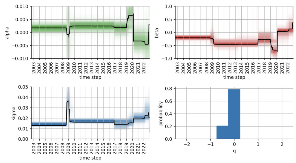
Figure 2: Inferred temporal evolution of the CAPM parameters with hindsight.
These plots reveal several insights: First, we notice an advantage of the bayesloop-type of regime-switching model, namely that we did not have to specify a number of regimes or there values. Rather, the chosen high-level model keeps the parameter values stable for prolonged periods until they jump abruptly to new, better fitting values. Second, we see that bayesloop not only infers the time-varying parameters , , and , but also the hyper-parameter q that is included in the high-level model (this is why the study instance is called HyperStudy above). The distribution of q does not "touch" the boundaries of our predefined interval, so no adjustments needs to be made. The same is true for , , and .
What can we learn from the temporal evolution of , , and ? The plots show that TLT features a positive alpha and negative beta for most of the time period that we analyze in this example, up to the Corona crash in 2020. During the financial crisis of 2008/2009, the parameter estimates are more uncertain, and our CAPM model does not fit the data well. This is nicely reflected by the increased parameter. The Corona crash induced a systematic change in market dynamics and pushed TLT to negative alpha values and zero beta. The model accurately captures the positive beta/correlation between stocks and bonds that we have seen in 2022.
This first overview tells us that the probabilistic, time-varying CAPM model works as intended and captures major macroeconomic shifts. Still, we cannot use the information contained in the plots above to derive trading decisions, because all data was passed into the inference process at once, so the estimates for e.g. 2008 are based on all data up until now and thus contains severe look-ahead bias. To overcome this issue, we repeat the inference process, but this time we use an OnlineStudy instance. In this type of analysis, we supply a series of individual data points to make sure that the resulting parameter estimates only take into account current and past data. Such online-inference methods can also be applied to fit probabilistic models on real-time data streams.
The following plots again show the temporal evolution of the time-varying parameters of the CAPM model, but without any look-ahead bias. Note that the hyper-parameter q that quantifies the likeliness of regime-switches is also slowly optimized over time. In contrast to the previous plots, the temporal parameter evolutions now appear more "erratic", mostly because the model needs to quickly correct parameter jumps that turned out not to be parameter jumps after seeing a few more data points. Still, the major shifts over time resemble the results that we got from the fit that included look-ahead bias:
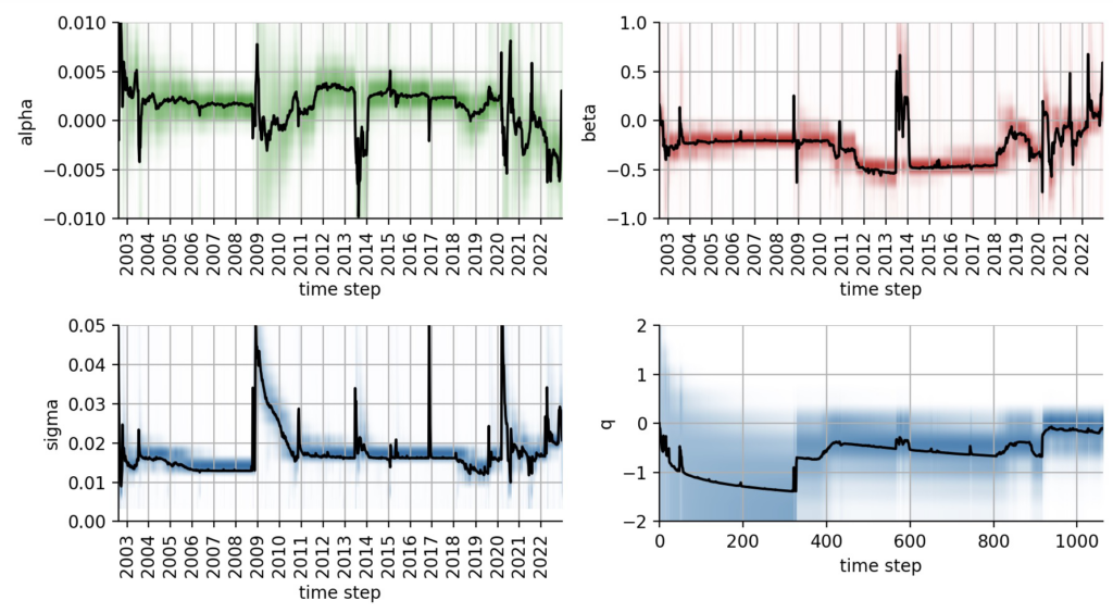
Figure 3: Inferred temporal evolution of the CAPM parameters without hindsight, using online parameter estimation.
Intuitive probabilistic indicators
From the fit of the probabilistic CAPM model, we have obtained the joint distribution of and for each trading week. Based on these distributions, we now want to build trading indicators that we can subsequently use to build a simple trading strategy. The "probabilistic attractiveness" of a financial asset can be summarized as follows: investors want to be certain that the asset has positive alpha (to generate excess returns), and they want to be certain that the asset has negative beta (to diversify from the market). Based on the distributions we have obtained, we can directly compute the probability that alpha is positive, and the probability that beta is negative :
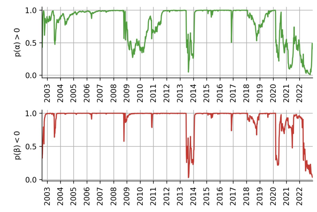
Figure 4: Intuitive trading indictors derived from the time-varying probability distributions of alpha and beta.
As we can see, TLT features multiple time periods in which it positive alpha and/or negative beta with high certainty. Note how asking for generates a curve that is easy to understand and has an intuitive meaning, whereas if we only cared whether , we would always worry about the uncertainty that is tied to the estimate.
From probabilities to trading decisions
To test the value of probabilistic trading indicator that we have defined above, we will devise a - admittedly very oversimplified - trading strategy. By default, we will be long-term SPY investors. However, if we are at least 95% certain that TLT provides positive alpha, we will switch everything we have to TLT. This strategy ignores beta for now and there is no allocation sizing, we either invest 100% in SPY or 100% in TLT. The plot below shows the resulting trading intervals:
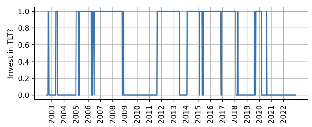
Figure 5: Allocation weight for TLT, based on the probabilistic alpha trading indicator.
Simple backtest
To simulate this strategy, we first compute arithmetic weekly returns from the log-returns we used during model fitting, then multiply them by the allocation weights (to decide whether to invest in SPY or TLT), and then compute log-returns again. Note that we shift the indicator by one week, so that trading decisions are always lagged by one week to not fall for any look-ahead bias again. Note also that we do not account for transaction costs in this simple example as the strategy trades rarely. The plot below shows that indeed, this simple strategy trades above TLT all the time and above SPY most of the time. Additionally, it greatly minimizes the overall draw-down during the financial crisis of 2008/2009 and during the Corona crash in 2020:
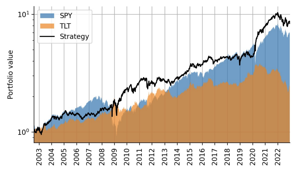
Figure 6: Trading strategy backtest in comparison to individual buy-and-hold portfolios.
Despite the over-simplistic switch between 100% SPY and 100% TLT investment, this strategy also outperforms the weekly-rebalanced 60/40 portfolio comprised of 60% SPY and 40% TLT:
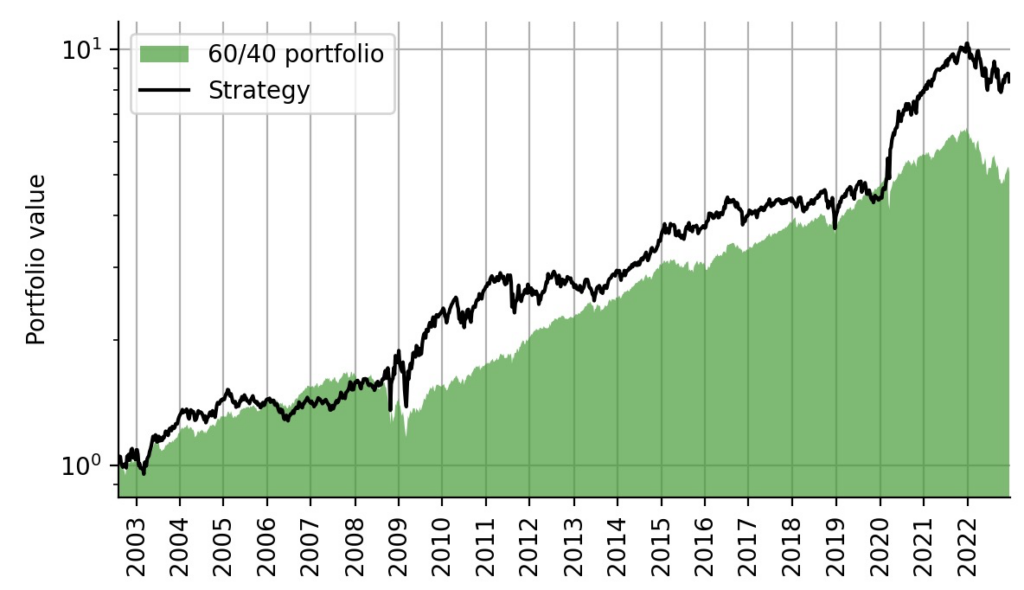
Figure 7: Trading strategy backtest in comparison to the classic 60/40 portfolio.
Volatility-matching via beta-scaling
So far, we have completely ignored the beta parameter of the CAPM model. Beta describes the risk/volatility of an asset relative to a benchmark. In our case the benchmark is the S&P500 index, realized via the SPY ETF. We could use the beta distribution is various ways to refine our trading strategy. For example, we could stop trading TLT if grows to large, as TLT then is no longer negatively correlated to SPY. Such an additional condition could protect us in recent market conditions in which stocks and bonds decline in unison. A high value of could for example indicate attractiveness of commodities, energy or other sectors. Here, we want to instead focus on a simpler use of beta: allocation sizing. The volatility of stocks is generally higher than the volatility of bonds, and this relation is captured by the mean value of our time-varying beta parameter, as displayed below:
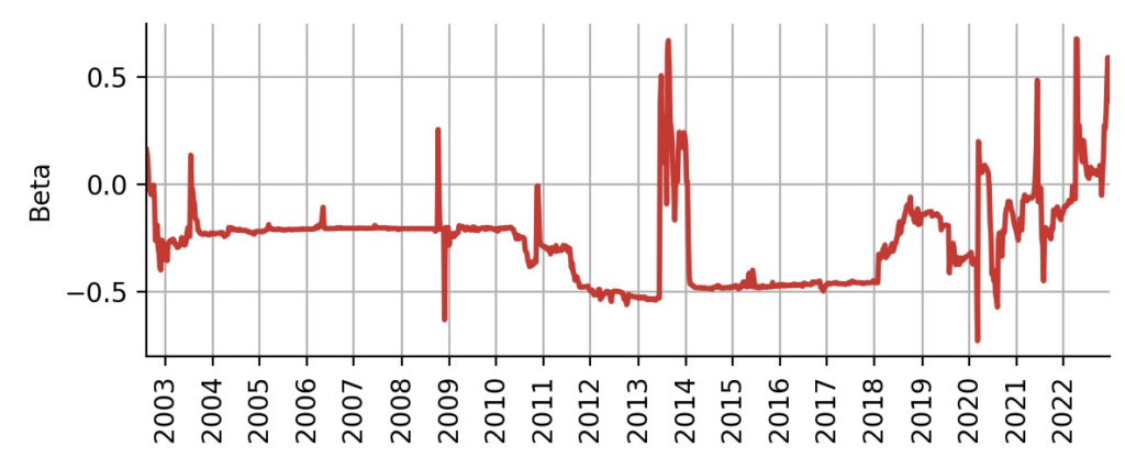
Figure 8: Inferred time-varying beta parameter.
In our original strategy, we assumed that we are SPY investors by default. This indicates that we are risk-tolerant up to the volatility value of SPY. Whenever the original strategy switched over to TLT, our investors' exposure to price fluctuations decreases because TLT has a lower volatility. Depending on the value of beta, we could thus not only invest 100% in TLT, but enter a leveraged position to (approximately) match the volatility of SPY and thus maximize the risk-adjusted excess return that we obtain through TLT's alpha at that time. A leveraged bonds-position can be realized e.g. via Futures contracts or via leveraged ETFs.
How to compute the leverage factor of the bonds position that we want to enter? If the current volatility of TLT is half of the volatility of SPY, we want to attain a leverage factor of 2, i.e. we invest double the money that we currently have. If the current volatility of TLT amounts to a third of the volatility of SPY, we want to attain a leverage factor of 3. Below, we compute this leverage factor, rounding to whole numbers to avoid over-adjusting the position week-by-week and capping the leverage factor at 1 the lower end at 3 at the upper end. The plot shows that most of the time, the beta estimates indicate that a high leverage factor is tolerable:
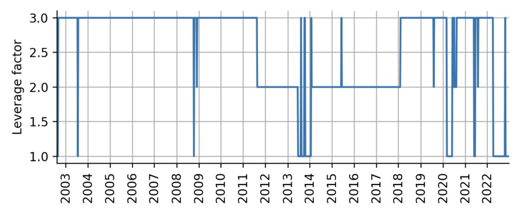
Figure 9: Leverage factor for the TLT position, derived from the inferred beta value of the CAPM model.
Finally, we can merge the allocation weights from the original strategy with the leverage factors that we have obtained from the inferred beta factor to backtest the improved strategy. As we can see, the volatility-matching of the TLT position greatly increased the excess returns of the strategy. Keep in mind, though, that again we did not account for increased transaction costs or margin costs for the leveraged position.
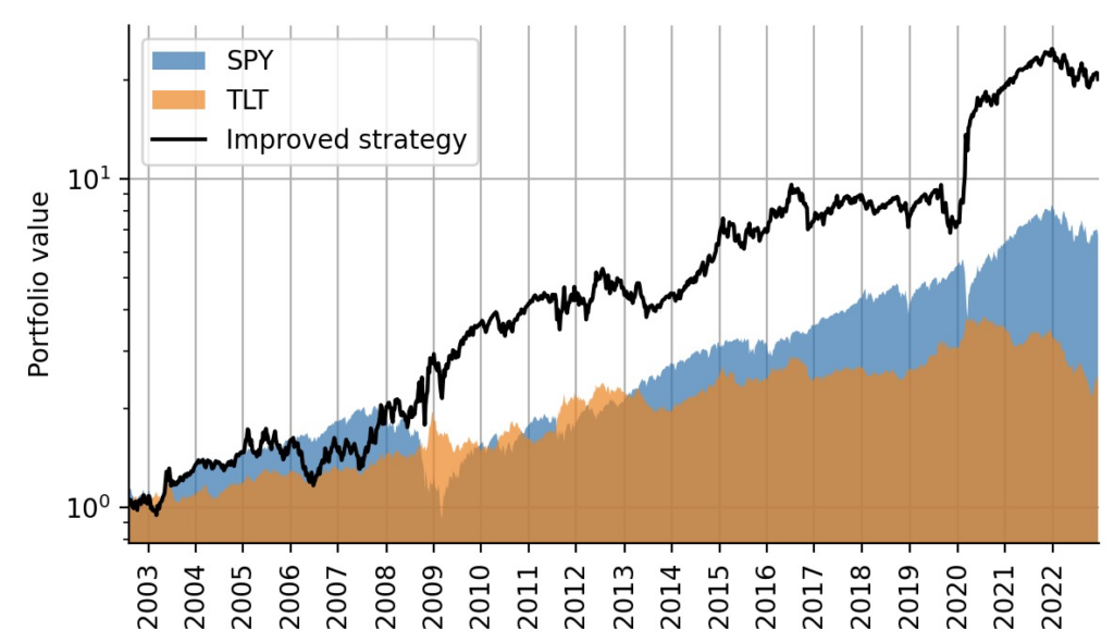
Figure 10: Improved trading strategy backtest in comparison to individual buy-and-hold portfolios.
Of course, this toy example can be extended in many ways, including more asset types beyond a broad index and long-term bonds, by implementing proper allocation sizing, by accounting for uncertainty due to the parameter, and so on…
Get notified about new blog posts and free content by following me on Twitter @christophmark_ or by subscribing to our newsletter at Artifact Research!
Related posts
Skewness: the fallacy of the expected return
In this post we will take a closer look at the expected return that is often stated for investments like stocks and other financial assets, or for certain outcomes in gambling. The point we want to convey is that the expected return is only valid for one period or a single “iteration” (say, one year, or one round of a game such as Blackjack), but that the expected return can be highly misleading for more long-term investments that involve continuous re-investing, i.e. compound interest. We will see that compounding introduces substantial positive skewness in the long-term return distribution. While this skewness certainly represents a beautiful property for building wealth in the long-term, it also renders the expected long-term return misleading as there is a high probability that one will not achieve the long-term expected return! We will learn that to correct for skewness, we need to use the geometric mean instead of the arithmetic mean that is used to compute the expected return – which will lead us to the Compound Annual Growth Rate (CAGR).
How heavy tails destabilize Markowitz portfolio selection
This is the forth and final post of a short series of posts on extreme events in financial time series. In the first post , we have introduced power-law theory to describe and extrapolate the chance of extreme price movements of the S&P500 index. In the second post , we took a closer look at how statistical moments may become infinite in the presence of power-law tails, rendering common estimators useless. In the third post , we have seen how infinite kurtosis makes GARCH risk models fail on out-of-sample data. In this post, we turn to Markowitz’s Modern Portfolio Theory and show how the heavy tails of financial return distributions drastically increase the uncertainty in portfolio allocation weights.
Why GARCH models fail out-of-sample
This is the third post of a short series of posts on extreme events in financial time series. In the first post , we have introduced power-law theory to describe and extrapolate the chance of extreme price movements of the S&P500 index. In the second post , we took a closer look at how statistical moments may become infinite in the presence of power-law tails, rendering common estimators useless. In this post, we will investigate the consequences of infinite moments by showing how the popular GARCH risk model almost perfectly describes in-sample data, but fails to extrapolate to out-of-sample data.