Skewness: the fallacy of the expected return
In this post we will take a closer look at the expected return that is often stated for investments like stocks and other financial assets, or for certain outcomes in gambling. The point we want to convey is that the expected return is only valid for one period or a single "iteration" (say, one year, or one round of a game such as Blackjack), but that the expected return can be highly misleading for more long-term investments that involve continuous re-investing, i.e. compound interest. We will see that compounding introduces substantial positive skewness in the long-term return distribution. While this skewness certainly represents a beautiful property for building wealth in the long-term, it also renders the expected long-term return misleading as there is a high probability that one will not achieve the long-term expected return! We will learn that to correct for skewness, we need to use the geometric mean instead of the arithmetic mean that is used to compute the expected return - which will lead us to the Compound Annual Growth Rate (CAGR).
What is skewness?
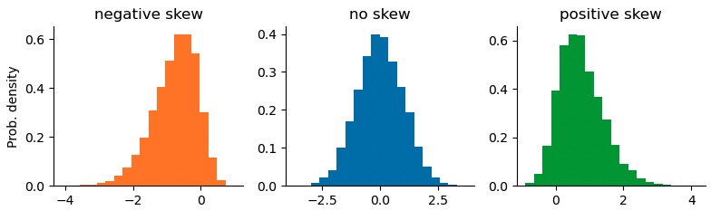
Skewness describes the asymmetry of a probability distribution - its lopsidedness. Skewness is defined as the third standardized moment of a probability distribution:
where is the mean, is the standard deviation, and is the expectation operator. Visually, positive skewness results in a longer right tail of the distribution, whereas negative skewness results in a longer left tail of the distribution. As skewness thus encodes information about extreme values in the tails of a distribution, it is important whenever the distribution represents payoffs or returns on investments: investors or gamblers prefer bets with a positively skewed payoff distribution as extreme positive payoffs are more likely than extreme losses. Likewise, negatively skewed payoffs are often associated with "hidden risk", as the longer left tail is not fully captured by risk estimates such as the standard deviation (volatility).
We can easily simulate skewed random numbers using the Python function scipy.stats.skewnorm:
In the following we will discuss how making repeated bets or re-investing of previous profits and losses create a positive skew in the final payoff distribution, and how we can properly evaluate what to expect from repeated bets in the long run.
Compounding as the source of positive skewness
Compound interest is gained by reinvesting the payoff of an investment in the next investment period. Instead of investments, you can think of this iterative process in terms of (sports) bets: you place a wager of $100 on a bet and you win, leaving you with $150. Instead of taking your $50 profit out of the game, you place a wager of $150 on the next bet. Even if the second bet has the same odds as the first one, the potential absolute profit (and loss) is now higher as your stake is higher. If you take a series of bets in which you have an edge (for example because you know your favorite sports team better than anyone else), you can expect to be right more often than wrong and thus you expect a positive payoff on average. As you re-invest everything in each new bet, you thus assume that your wealth will increase exponentially as your wager increases with each new bet!
In the following, we will use simple Python code snippets to simulate such a series of bets in which you have a positive expected payoff (on average, you win more than you lose) and in which you always re-invest everything. While our hypothesis of exponential growth is correct in this case, we will see that the expected return (or expected payoff) after several bets will be increasingly misleading and that there is a high probability that we will actually gain less than what the expected return suggests.
First, we define the (very favorable) bet that we are going to accept again and again. Here, prob denotes the probability of the two different outcomes, and payoff denotes the payoff per unit wager that one gains (or loses) depending on the outcome. The bet has two outcomes with equal probability of 50%, and the payoffs are 100% in one case and -50% in the other case. This means that we will either double our wager or lose half of it each time we accept the bet:
In terms of absoulte payoff, this bet offers a great edge: if you risk 100 or lose $50 with equal probability. We can summarize this edge by computing the expected return or expected payoff that is calculated as the probability-weighted sum of all payoffs:
The expected return tells us that this bet has a positive net outcome of 25%. The expected return is often stated in evaluations of financial assets, to help in the process of portfolio selection. As we will see later, the S&P500 index has an expected annual return of 8.8% (including dividend payments and adjusted for inflation). But what does that mean for a long-term investor? The expected return summarizes one single bet, one single investment period, but can we use the expected return to extrapolate to a series of bets or longer investment periods with repeated re-investments of returns? The answer is yes and no: while the expected return indeed holds for repeated investments, the probability of actually realizing the expected return decreases drastically with the number of investment periods - because of skewness!
Let us investigate this effect step by step. Below, we calculate the expected compound return of simple bet that we have defined above. In particular, we assume that we start with $1000, and that we make a series of 8 bets, all of which have 25% expected return:
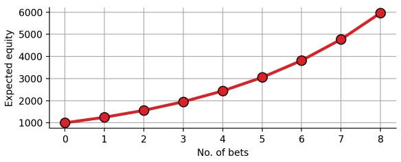
As expected, compounding the expected return results in a exponential equity curve. At each iteration, we gain 25% and subsequently re-invest everything. After making the bet 8 times, we have increased our equity by 6-fold. However, note that the formula we have used above only takes into account the expected return, but not the individual payoffs! This means that the curve above looks the same for all of the following bets, simply because all of them have the same expected return of 25%:
While you might be willing to make the original bet that results in a maximum loss of 50% of your wager, you most certainly will not risk 99% of your wager for the opportunity to win 149%. If you lose the latter bet only once, you need many many wins to make up for the loss again. Clearly, the expected return misses this critical aspect of risk taking, because it only focuses on a single bet, not on a series of repeated bets.
The expected compound return explicitly ignores uncertainty and draw-downs. To overcome this issue, we turn to a Monte Carlo experiment and simulate 100,000 individuals who each make 8 consecutive bets as the one that we defined in the beginning (50% chance of doubling the wager, 50% chance of losing half of the wager):
Below, we overlay 1,000 of these simulated equity curves with a transparent shading. The resulting figure show a branching binary tree that illustrates the different sequences of winning and losing individual bets. The darker a certain path, the more probable it is (example: winning 4 bets and losing 4 bets is more probable than winning or losing all 8 bets). In addition to the branching binary tree, we plot the expected equity that we have plotted above. Note that we use a logarithmic scaling of the y-axis, such that the plotted distance between 10 and 100, or 100 and 1,000, or 1,000 and 10,000 is identical. This type of scaling is always helpful when one is visualizing a multiplicative process (such as compound returns):
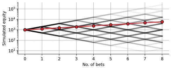
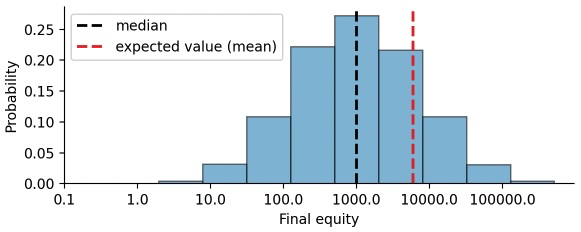
The simulated equity curves nicely illustrate the risk that is inherent to the bet, which is ignored by the expected equity value. Let us take a look at the distribution of potential final equity values after making 8 consecutive bets:
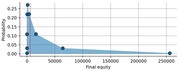
Each point in the plot above corresponds to a certain number of won bets, resulting is a highly skewed distribution. The substantial, positive skewness is created by compound payoffs: In the (unlikely) case that we win all 8 bets, we are able to double our wager for each new bet. This doubling of the wager results in exponential growth and a final value of 256 times the initial wager:
This positive skewness of the equity distribution after repeated bets/investments is the key to building wealth via long-term investments. However, we also see that the expected value of the distribution (red dashed line) does not really capture any characteristic point of the distribution, it seems oddly out-of-place. To get a better view on the equity distribution, we plot it again, but this time we scale the x-axis logarithmically:
On a logarithmically scaled x-axis, the equity distribution looks like the ubiquitous, symmetric, bell-shaped normal distribution (also called Gaussian distribution). Indeed, compound returns (or equity values after repeated bets) follow a so-called log-normal distribution, because the potential outcomes are the result of multiplying individual return values. If returns added up instead of being multiplicative, we would end up with the normal distribution. With this visualization, we get some insight on why the expected equity is positive: the log-normal distribution is symmetric around the initial wager ($1000) on a logarithmic scale, but the expected value is calculated on a linear scale, resulting in a right shift because 10,000 is further to the right of 1,000 than 100 is to the left of 1,000.
The equity distribution of our series of bets reveals that there is significant uncertainty in the final payoff, spanning multiple orders of magnitude. Relying on the fact that the expected value of this distribution is positive will not get you far as an individual risk taker! You only have one chance, one lifetime to make bets and invest, and one big draw-down may take your whole lifetime to recover. We can easily convince ourselves of this short-coming of the expected value by computing the probability that our final equity is smaller than the expected equity:
In more than 85% of all simulations, the final equity was smaller than the expected equity! This may sound counter-intuitive at first but think about it this way: The positive skewness of the distribution creates a thin but long tail towards very high equity values. This means that in the rare case in which the equity is larger than the expected value, it is waaaaay larger. But in most cases, it will stay below the expected value. The expected value thus is only a helpful metric in cases where you can split your wager into many independent wagers. Say that instead of putting up a single wager of 1 to 1000 people and they make the 8 bets for you and give you back the payoff afterwards. The resulting payoff will be much closer to the expected value because you can average winners and losers.
If we cannot split up our wager/investment into many independent bets, we need to find an alternative metric for the expected compound return that correctly reflects the risk that an individual takes by entering the series of bets. One common example is the median. The median is the value that separates a list of values into a lower half and an upper half of equal length. Put differently, there is at least a 50% chance that the final equity of an individual will be equal or larger than the median. The median equity in our simulation is:
Interestingly, the median equity of our simulations equals the initial wager! For an individual risk taker, this means that there is only a 50% chance of making any profit at all in the series of 8 bets, despite the fact that each bet has a positive expected return of +25%.
Arithmetic and geometric average
The counter-intuitive co-existence of the positive +25% expected return and the pure-luck 50% chance of making any profit in the serial bet above can be further elucidated in the context of the arithmetic mean vs. the geometric mean. In the case of equal probability for all possible returns (as in our case), the expected return is computed as the arithmetic average :
This additive combination of returns corresponds to the process of diversification, i.e. if you split your wager across many people who each make the bets independently. That is why expected values are commonly used by insurances, for example to estimate the fees that are necessary to cover expected damages. Car accidents generally happen independently of each other, so that the insurance company can estimate an expected damage based on the number of cases and their amounts of damage from a large pool of insurants.
While the insurance can average out the effect of many parallel bets, an individual risk taker usually has to make bets in a sequential manner, and a large loss may require many subsequent wins to break even. This sequential risk taking that involves re-investing profits and losses is described by the geometric average . The geometric average of all possible returns of a bet is computed as:
In our case, the geometric average is:
The geometric average of 1.0 indicates that by repeatedly making this bet with re-investing profit and losses, we will get back 100% of our wager on average, and thus will not win on lose on average, as the median suggested. Always calculate the geometric mean if you make single bet/investment repeatedly. Note that the geometric mean can also be stated in terms of log-returns:
Computing the log-returns of our example bet, we recover the symmetry that explains why there a 50/50 split between making profit or losing on this bet if played repeatedly:
There is another interesting property of using the geometric mean: assume that one outcome of a bet is bankruptcy, i.e. with a very small probability, you lose everything. If this probability is veeeery small compared to all the other outcomes, it will hardly affect the expected value (or arithmetic average). But since
the geometric average will immediately become zero, regardless of how small the probability of bankruptcy is! This again shows that the geometric mean evaluates the outcome of making a bet repeatedly, infinitely often to be exact.
Basic hedging: store of value
Our original toy bet was designed to include a 50/50 chance of doubling the wager or losing half of the wager:
If someone offered this bet to you after you have read the previous paragraphs, you might find yourself in a tough spot: the expected return is positive, but repeatedly taking this bet and re-investing profits and losses leaves you with a 85% chance of losing after just 8 rounds. Intuitively, you probably know the solution to this problem: Given the inherent risk of the bet, you would probably not wager everything you have on the bet at once, and you may also not re-invest all profits immediately. But what fraction of your total bankroll do you leave as a store of value, and what fraction do you wager?
To answer this question, we again simulate 100,000 possible equity curves based on the outcome of 8 sequential bets, but this time we leave a fraction of 50% of our equity as a store of value and only wager the other half in each bet. This results in effective payoffs that are smaller than in the original bet as we also take on a smaller risk:
Compared to the expected equity after the full-sized bets, the expected equity after 8 bets with a reduced 50%-wager is less than half:
However, do not let the expected value mislead you. As we have learned above, the median of the equity distribution is a much more realistic performance estimate. For the full-sized bet, the median equity was equal to the initial wager. By reducing risk, however, we are able to increase the median equity! In particular, 50% of all participants made more than 60% profit on the series of bets:
By reducing the wager, we also reduce the skewness of our payoffs. This in turn renders the expected equity more realistic, and "only" 64% of all participants attain a final equity value below the expected value (compared to 85% in case of the full-sized bet):
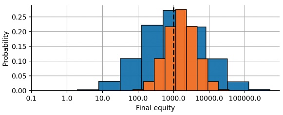
To visualize the difference between the full-sized bet and the reduced 50%-wager, we plot the equity distribution after making 8 bets. As we can see, the reduced bet yields a more narrow, but also right-shifted distribution. This example shows how one can use a basic store-of-value hedge to reshape the return distribution of a bet or an investment.
At this point, one might ask what the optimal "hedge ratio" is, i.e. what fraction of equity to wager and what fraction to leave unused as a store-of-value to obtain the maximal median equity after the series of 8 bets? We can easily simulate different hedge ratios and then plot the respective median equity:
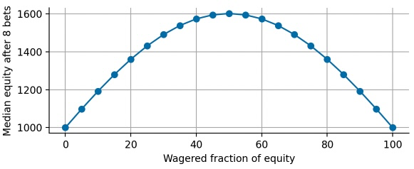
Indeed, we find that our initial guess of leaving 50% of our equity as a store-of-value maximizes the median equity after the series of bets. This optimal bet is also called Kelly bet (or Kelly strategy, Kelly criterion) that determines the optimal bet size to maximize the compound return of a bet or investment:
with:
- is the probability that the investment increases in value.
- is the probability that the investment decreases in value ().
- is the fraction that is lost in a negative outcome. If the bet loses 10%, then .
- is the fraction that is gained in a positive outcome. If the bet wins 10%, then .
You can easily evaluate this formula for our bet used in this example:
Compound Annual Growth Rate (CAGR)
The series of bets discussed above represents a rather abstract, extreme example of a skewed bet. However, the lessons we have learned about arithmetic mean, geometric mean, expected values, and median payoffs can be directly applied to real-world investment cases such as long-term index investing. In this section, we will apply the concepts we have learned so far to return data of the S&P500 index.
The following histogram shows the frequency of annual percentage returns of the S&P500 index over the last 125 years (including dividend payments and corrected for inflation), ranging from -38% during the Great Depression to +57% in the mid-fifties.
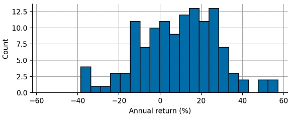
Calculating the expected return as the arithmetic mean of the annual returns as a first naive performance estimate, we find that the S&P 500 yields approximately 8.8% per year:
The average annual percentage return, also called the expected return, is 8.8% after adjusting for dividends and inflation. Certainly not bad! If you invest $100k, that is $8.8k of passive income per year on average. However, investing in an index like the S&P500 is often done as part of a long-term investment strategy, so you do not take the $8.8k out of your portfolio every year, but you reinvest your profit and let it compound over many years to accumulate compound interest.
At this point, you might be tempted to do the following calculation: After investing $100k for one year, you have $108.8k (on average), you reinvest the $108.8k, and after the second year you expect to have $108.8k1.088$118.4k. The compound interest made you $9.6k instead of $8.8k in the second year. You continue to reinvest for a total of 50 years. The final ending wealth of compounding the expected annual return 50 times can be calculated by
After 50 years, you expect to have accumulated $6.7M based on the initial investment of $100k, a 67-fold increase! Below you can see a chart of compounding the expected annual return as a function of the number of years invested:
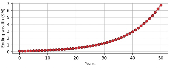
Looking at this idealized exponential growth, you might wonder whether you can really expect such an outcome, right? In reality, you do not get the average 8.8% growth each and every year, but you experience a wide range of outcomes, from -38% to +57% in the extreme cases. Indeed, we will proceed to show that simply compounding the expected return can be highly misleading, or putting it more specifically: While the compounded expected return as calculated above is still the correct expected return for the 50-year period, the probability of achieving this return (or better) is much smaller than you might expect!
To illustrate this, let us simulate many different "futures" of the S&P500 index. Imagine that we have a 125-sided die that we can roll to obtain a random annual return from our 125-year history of the S&P500. To simulate one single hypothetical future 50-year investment period, we roll our die 50 times. Of course, this assumes that the probability distribution of the annual return will not change in the future - certainly an oversimplifying assumption - but calculating the expected return from past values does the same thing. Now we let the computer roll our 125-sided die a few million times, to create 100,000 possible future 50-year series of annual returns. For each series, we then compound the returns to obtain the wealth of the investor over time, just like the red line in the graph above. The following graph shows just 100 of the 100,000 simulated hypothetical investments:
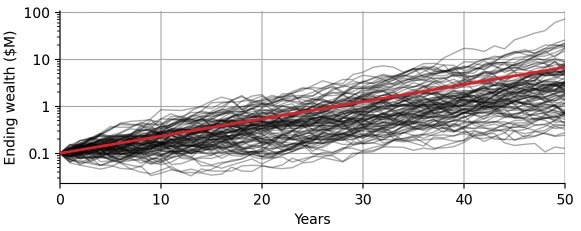
Each black line corresponds to a different hypothetical period of 50 years, sampled randomly from the true history of the S&P500 returns. Note how much variance we now notice: Some of the simulations take 30 years to break even after initial losses, whereas others almost reach $100M ending wealth. Note that we have switched the y-axis to a logarithmic scaling to better visualize all simulations together. The red line you see is the compounded expected return that we have displayed in the previous graph, ending at $6.7M after 50 years. The red line is now a straight line instead of the an exponential curve because of the logarithmic scaling. Comparing the black and the red line, we see the following important differences:
- The compounded expected return completely ignores variation. For the individual investor, however, this variation is what it's all about: we only have one life, one 50-year period to invest, we cannot average over 100,000 lifes to obtain the expected outcome. We need to look for investments for which almost all black lines show the desired minimal outcome!
- There are more black lines below the red line than above, indicating that the red line over-estimates the outcome. The red line is still the correct arithmetic mean of all the black lines, but for the individual investor who only has one life, the arithmetic mean is meaningless (no pun intended), as she cares more about probability. The individual investor needs to have e.g. 95% confidence that the investment will provide enough compound interest to retire after 50 years, i.e. 95% percent of the black lines need to provide the minimally needed amount to retire. That makes the individual investor sleep well at night, not the expected return!
Let us quantify those statements in more detail. Based on the 100,000 simulations we ran, 73.4% came out below the $6.7M that the compound expected return suggested, so in approximately 3 out of 4 cases you get less than what the compound expected return suggests!
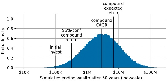
But what result can we expect with a high probability? What is a lower boundary of wealth that we can expect after an investment period of 50 years? This question is highly relevant for many people who use broad index investments for their retirement funds. We can calculate a very conservative estimate by choosing a low percentile of the simulated return distribution. For example, the ending wealth will equal or greater than the 5th percentile with 95% probability:
Investing $100k in the S&P500 will leave you with at least $322k after 50 years with 95% probability. These conservative estimates help to obtain an understanding of the risk of large draw-downs and can help in portfolio selection whenever there are set minimum amounts of equity needed at the end of the investment period.
In our toy example above, we found that the median return provides a more robust performance indicator compared to the expected return. In finance, the median return is also called the Compound Annual Growth Rate (CAGR), and it is often computed as the arithmetic mean of the *log-*returns, just as we have discussed above:
The CAGR of the S&P500 over the last 125 years is 7%, almost 2 percent points below the expected annual return. Note that the CAGR is a metric that we can easily compound to obtain an estimate of the median return after 50 years:
Compounding this CAGR over 50 years, we get an expected ending wealth of $2.9M. We will attain this ending wealth or larger with a probability of 50% - this is the "centering" property of the CAGR.
Finally, let us take a look the distribution of possible ending wealths that we may attain by investing $100k in the S&P500 for 50 years, and annotate all the different metrics we have discussed so far:
The content of this blog post is part of an in-depth course on risk mitigation that is offered as an online or on-site seminar by Artifact Research. Reach out in case you are interested in participating!